CS 541: Deep Learning
Convolution neural networks (CNNs)
Section titled “Convolution neural networks (CNNs)”Why FCNNs fail
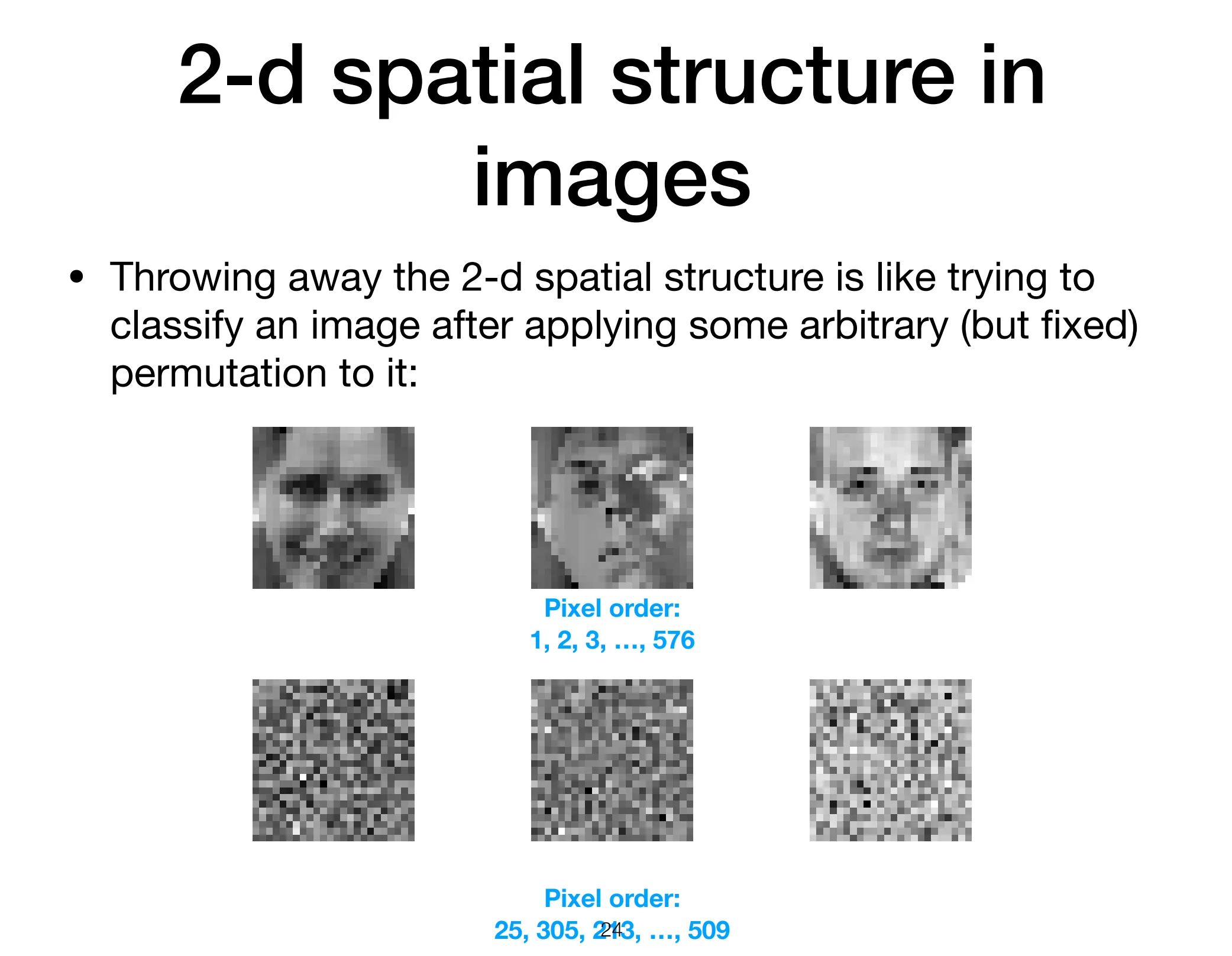
Section titled “Why FCNNs fail”The problem of FCNNs when applied to images is that the same pixels, while representing the same object could shift, warp, deform a bit through the lens of a camera. From the neural network’s perspective, totally different pixels are fed into the neurons -> A tiny shift in the input image can result in arbitarily different activations in the hidden layers.
Also the activation of each neuron in a layer is independent of the activations of every other neuron in the same layer. The neurons don’t communicate like in attention. In other words, the hidden layers have no spatial structure and the ordering of the neurons in a layer is meaningless. This preservation of spatial structure is crucial for image processing.
Images contain the same visual features (lines and corners of different colors) at many locations and scales -> no need that parameters to describe them.
Intuition: CNNs is an extreme form of weight sharing, forcing the neural network to have fewer degrees of freedom. This is a very strong form of regularization.
Convolution
Section titled “Convolution”Filtering with convolution
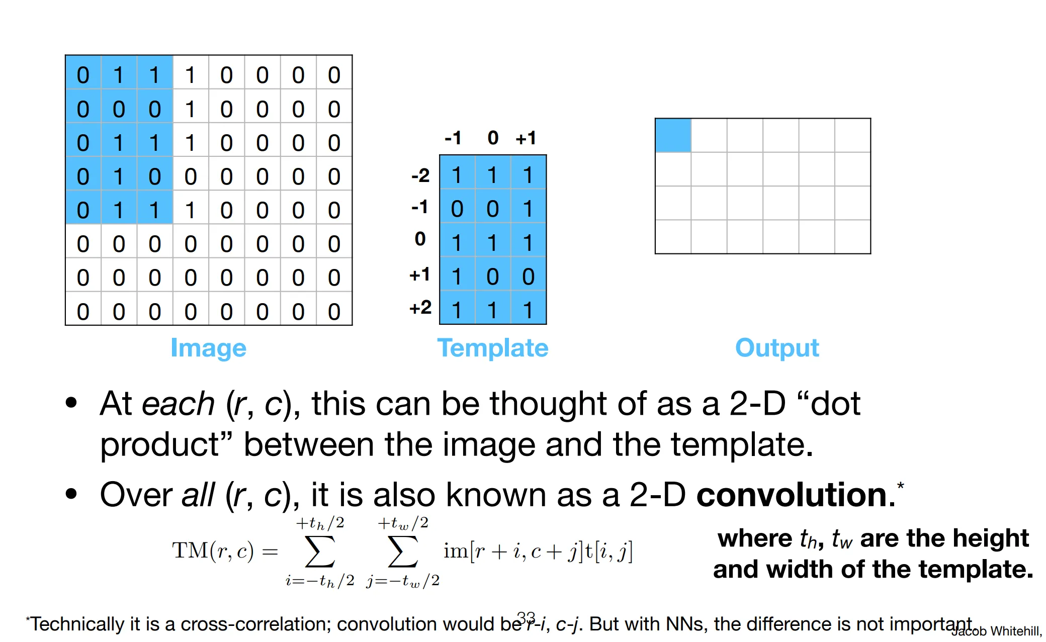
Section titled “Filtering with convolution”Inspired by the old CV strategy called template matching: we create one “template” matching the object we are looking for and slide the template across every location in the image and see where the image and template best “match”.
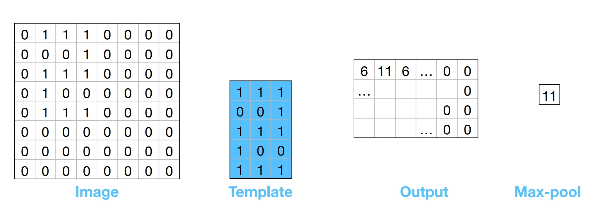
To classify the image without caring its location in the image, we can just compute the maximum of the output. This is called maximum pooling (max-pool).
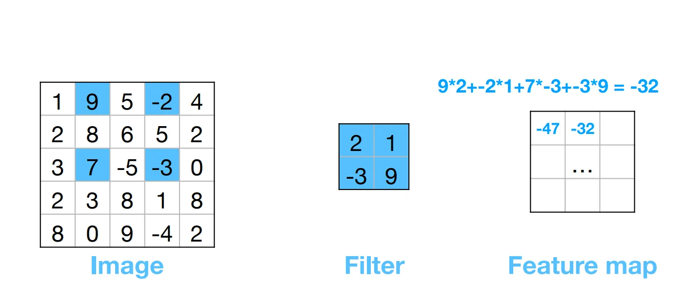
These templates are also called filters, or kernels. The output image is more commonly known as a filter response, or feature map.
To preserve the input image, we can pad the input image. We can also apply the template with a stride of k pixels (take k steps at a time when convoluting). To expand the spatial extent of the filter without increasing the number of parameters, we can dilate it by adding spaces between filter elements -> dilated convolution (à trous).
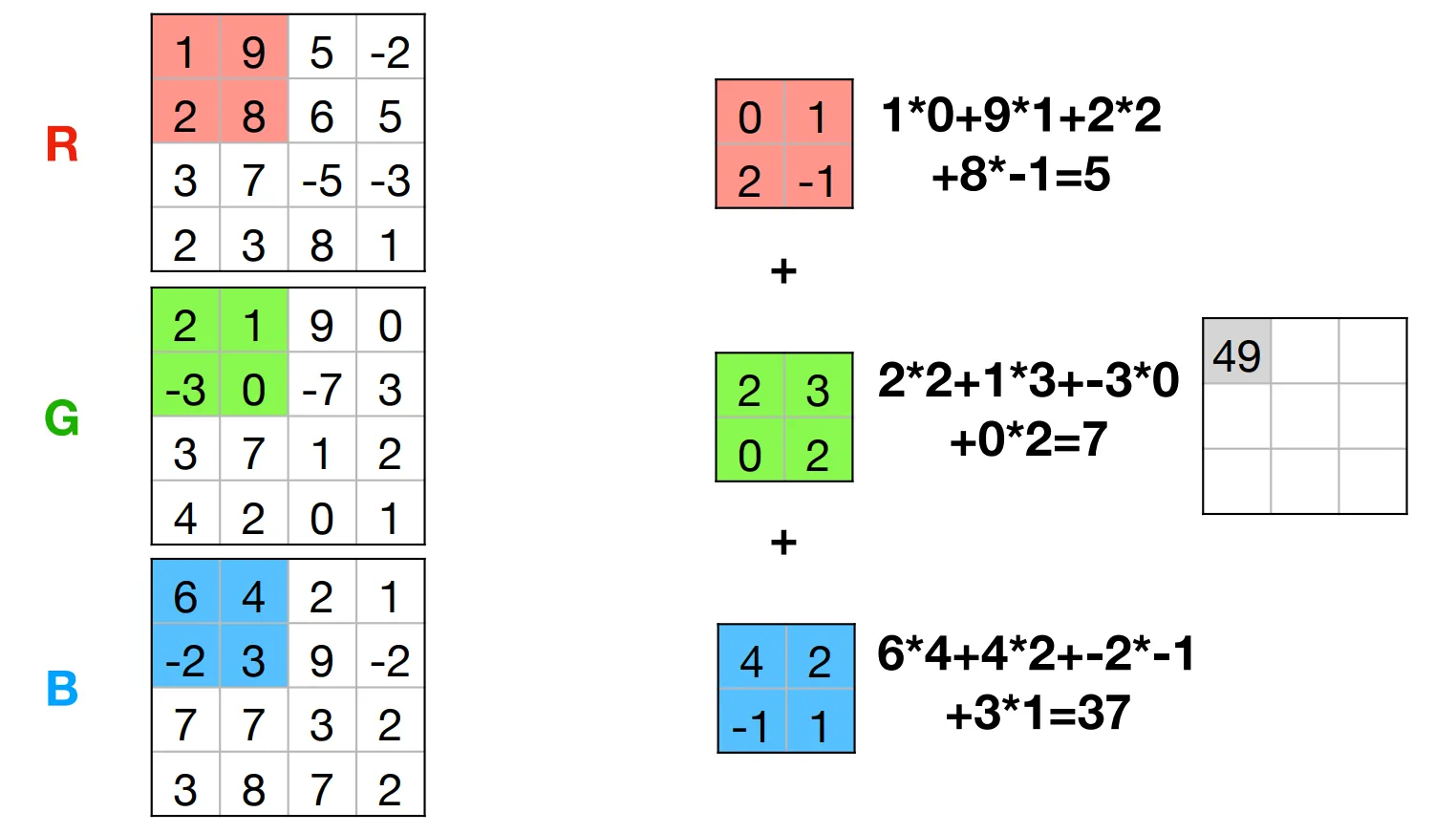
3D convolution is the same, you sum up the output of each channel of the filter to get the filter’s output.
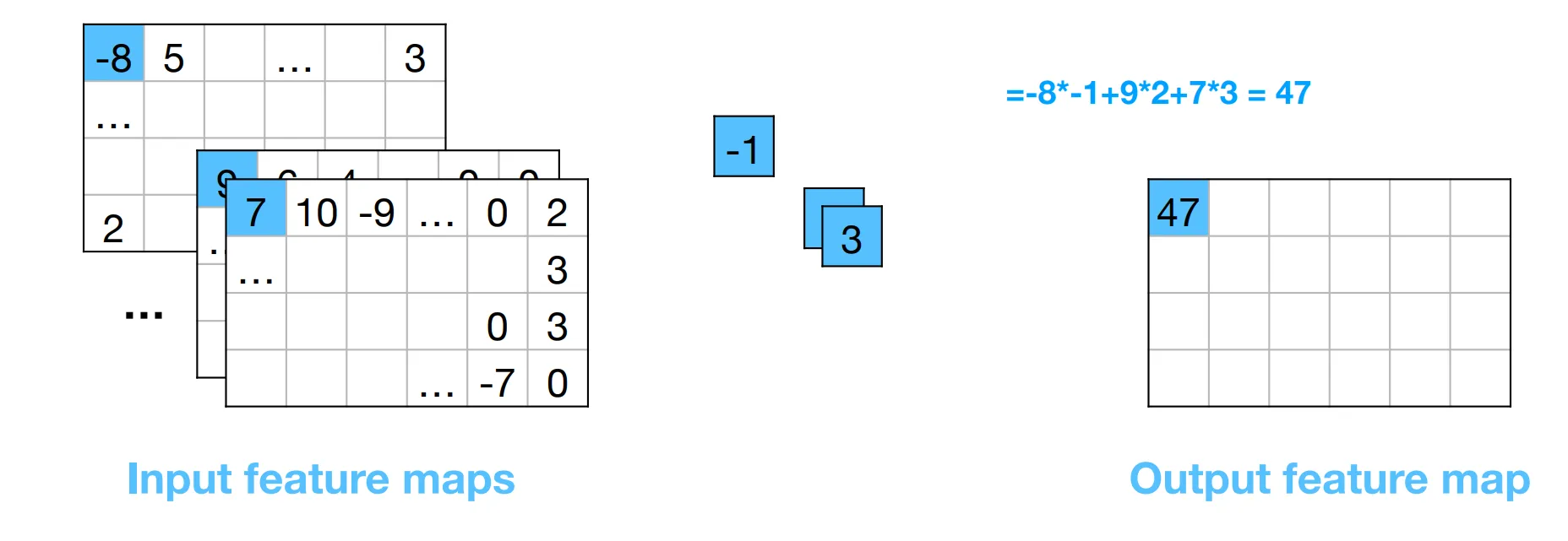
Hence 1D convolution is just a weighted sum of the input feature maps.
Summarizing with pooling
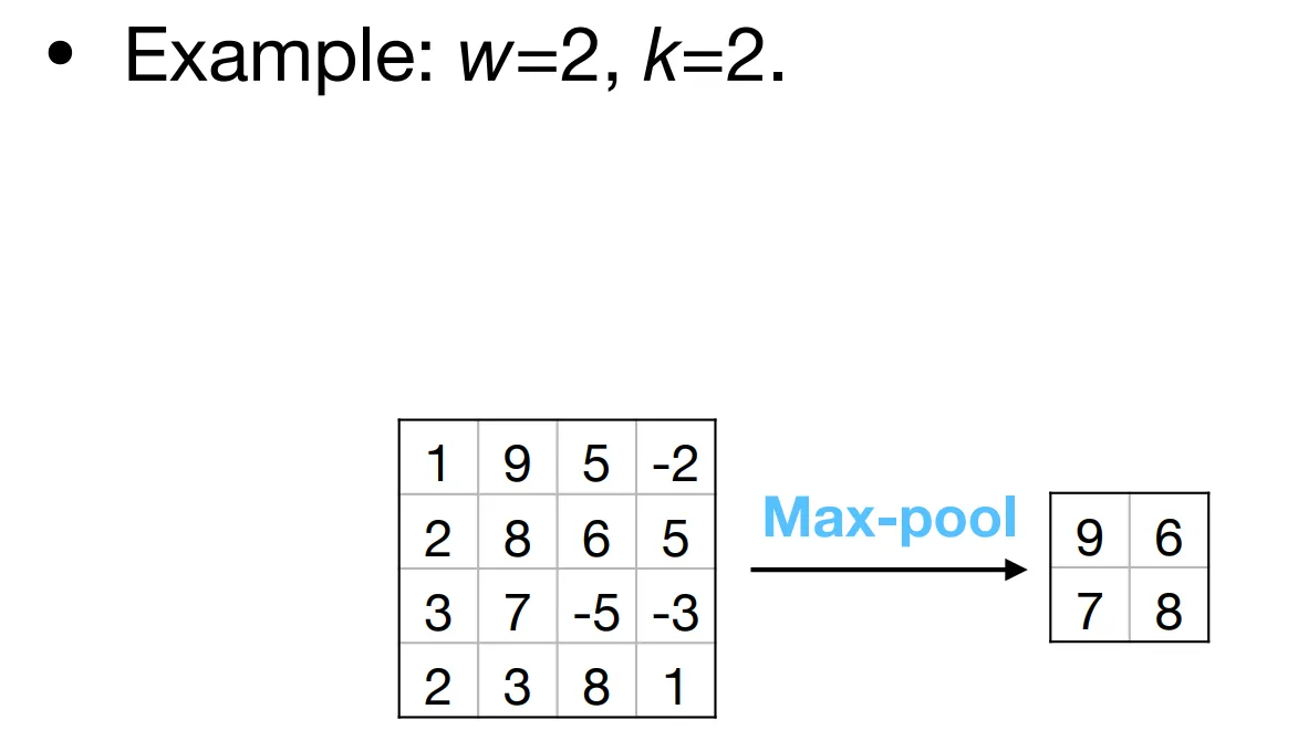
Section titled “Summarizing with pooling”Instead of pooling over the whole image, we can pool over small sub-regions of size w. We can also use a stride of size k. (We could also use padding.)
Convolution neural networks
Section titled “Convolution neural networks”CNNs are networks that consist of 1+ convolutional layers and usually some non-convolutional layers at the end. The filter parameters instead of chosen by hand in template matching, are trained with back-propagation.
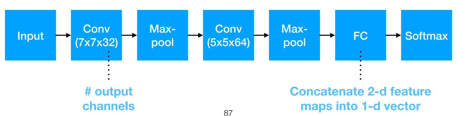
Composition of CNNs:
- Multiple convolutional layers
- Pooling layers in between some of the convolutional layers
- FCNN layers at the end for classification
- Non-linearies between each layer
- Number of channels in earlier layers is small, whereas the spatial resolution is high. The filters detect low-level features, e.g., edges & corners of different orientations & sizes.
- Number of channels in later layers is large, whereas the spatial resolution is low. The filters detect high-level features such as object parts.
Receptive fields
Section titled “Receptive fields”Receptive field of a neuron is the region in the input image that can affect the neuron.
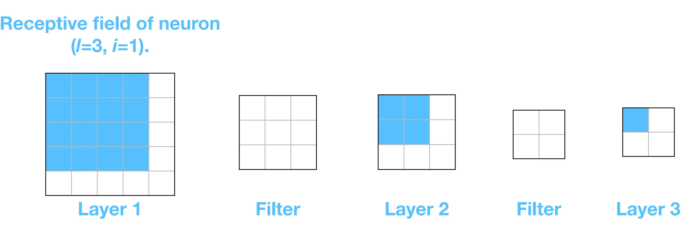
Intuition: The deeper the network, the larger the receptive field of the neurons in the later layers. The later layers’ neurons essentially pay attention to the entire input image at some point.
Properties of convolution
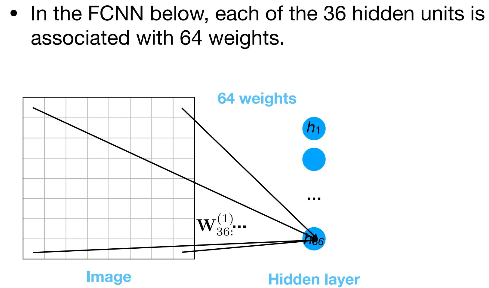
Section titled “Properties of convolution”CNNs are a special case of FCNNs
Section titled “CNNs are a special case of FCNNs”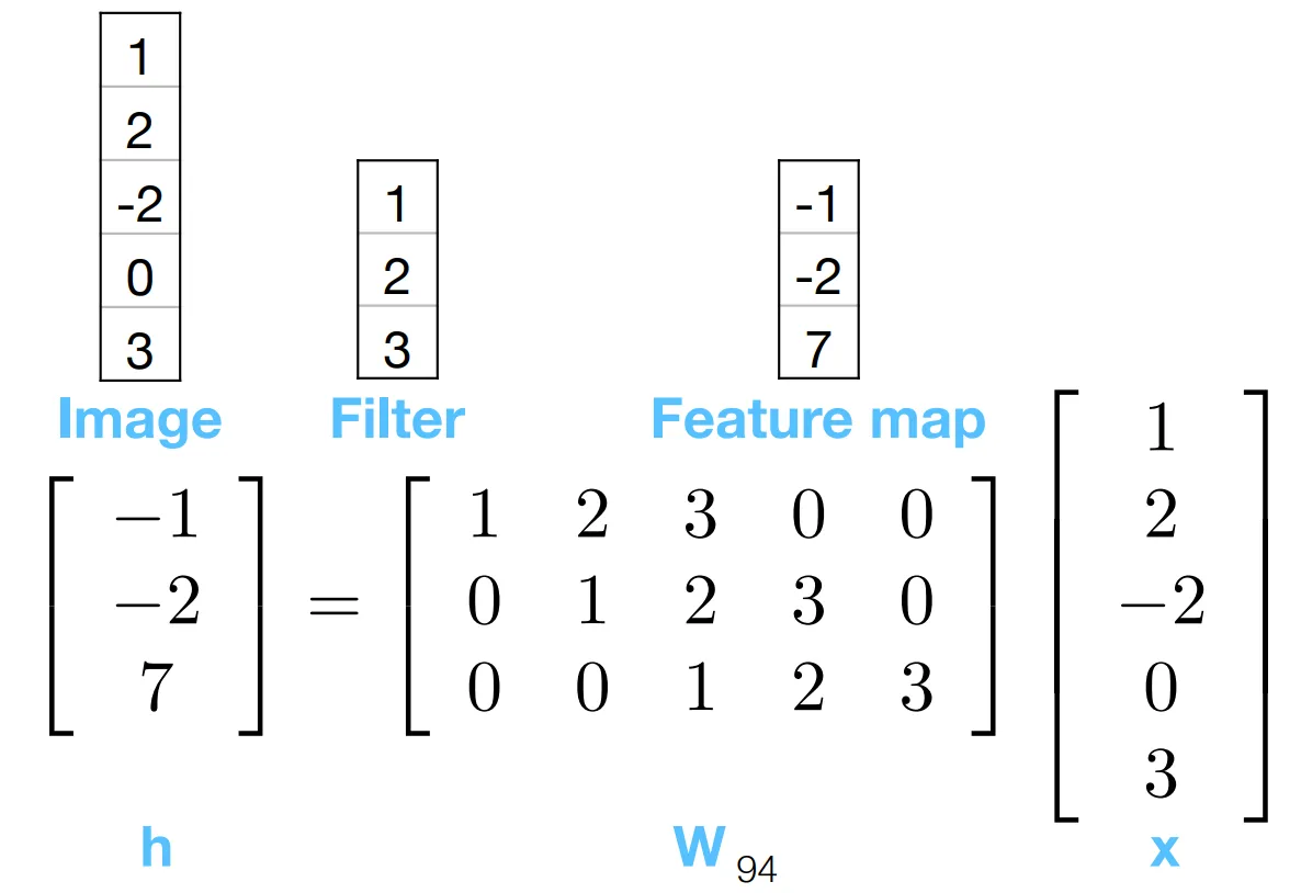
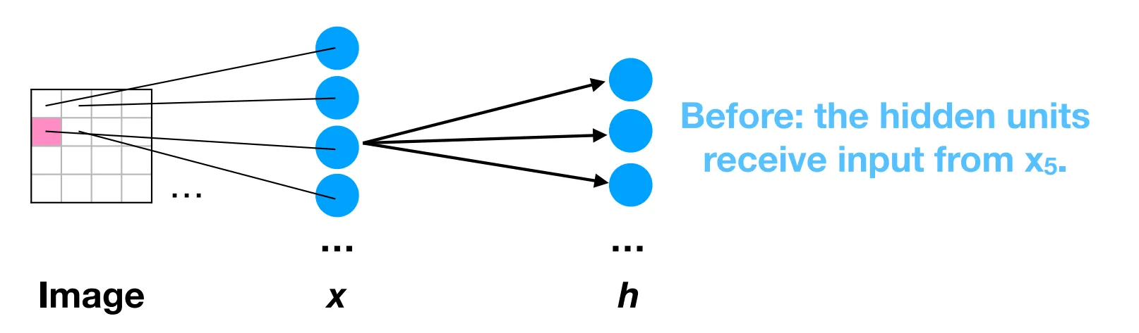
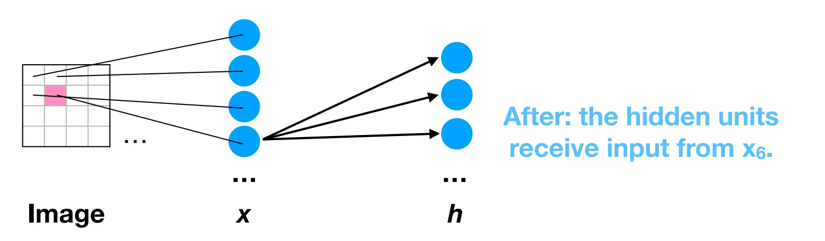
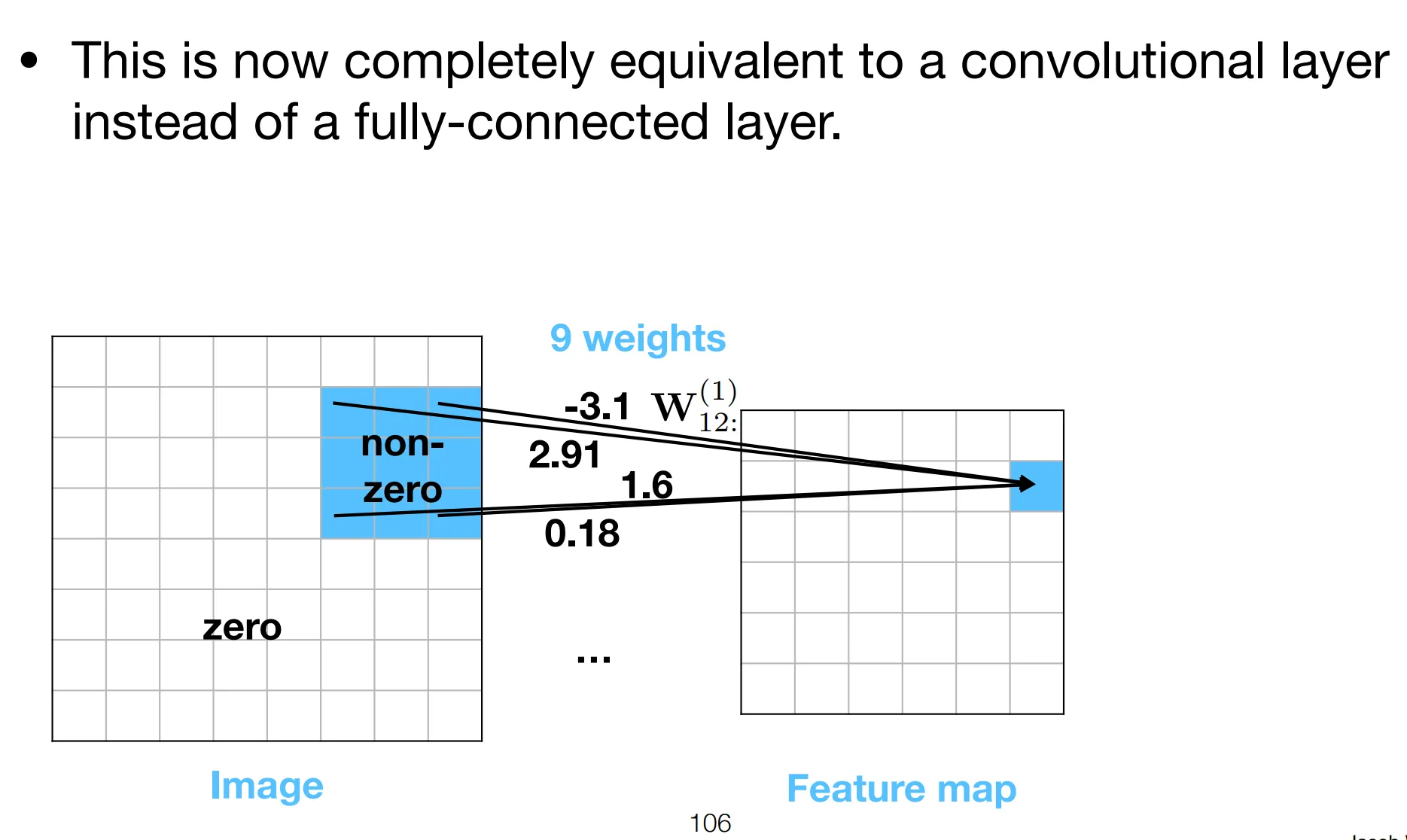
Convolution is a special case of the general feed-forward neural network.
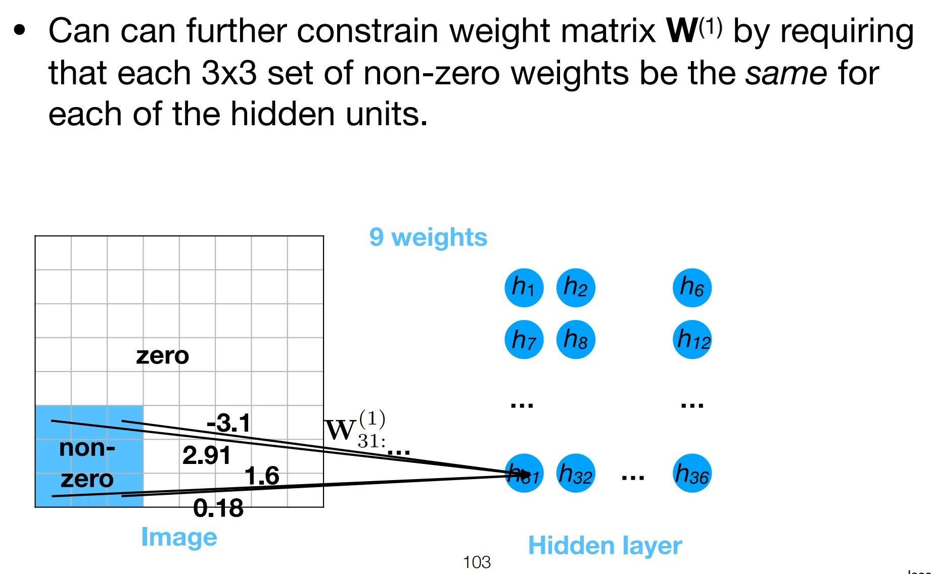
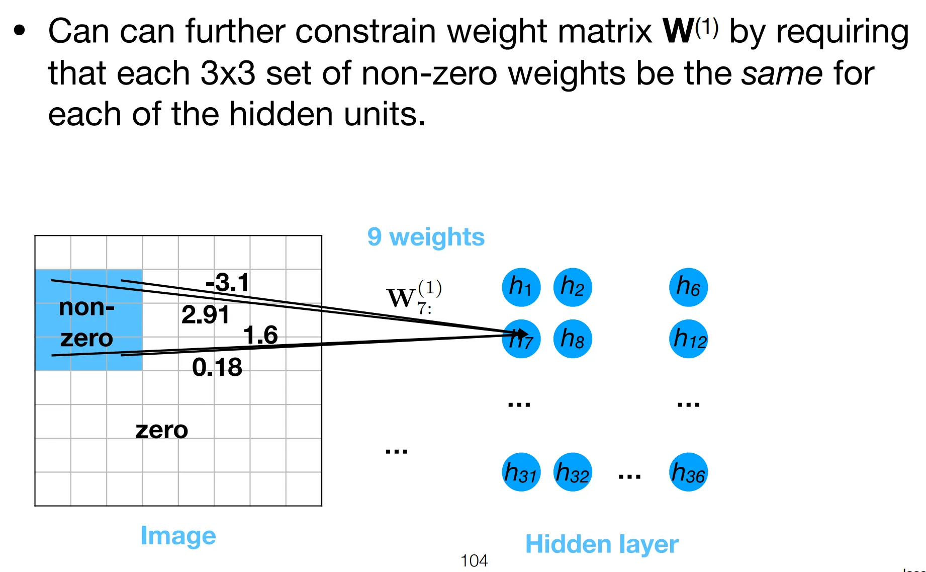
Notice how the weights only has 3 free parameters, either equal to the filter’s elements or 0. This is the strong regularization effect refered to above.
Now we prove FCNNs with certain constraints, are in fact CNNs.
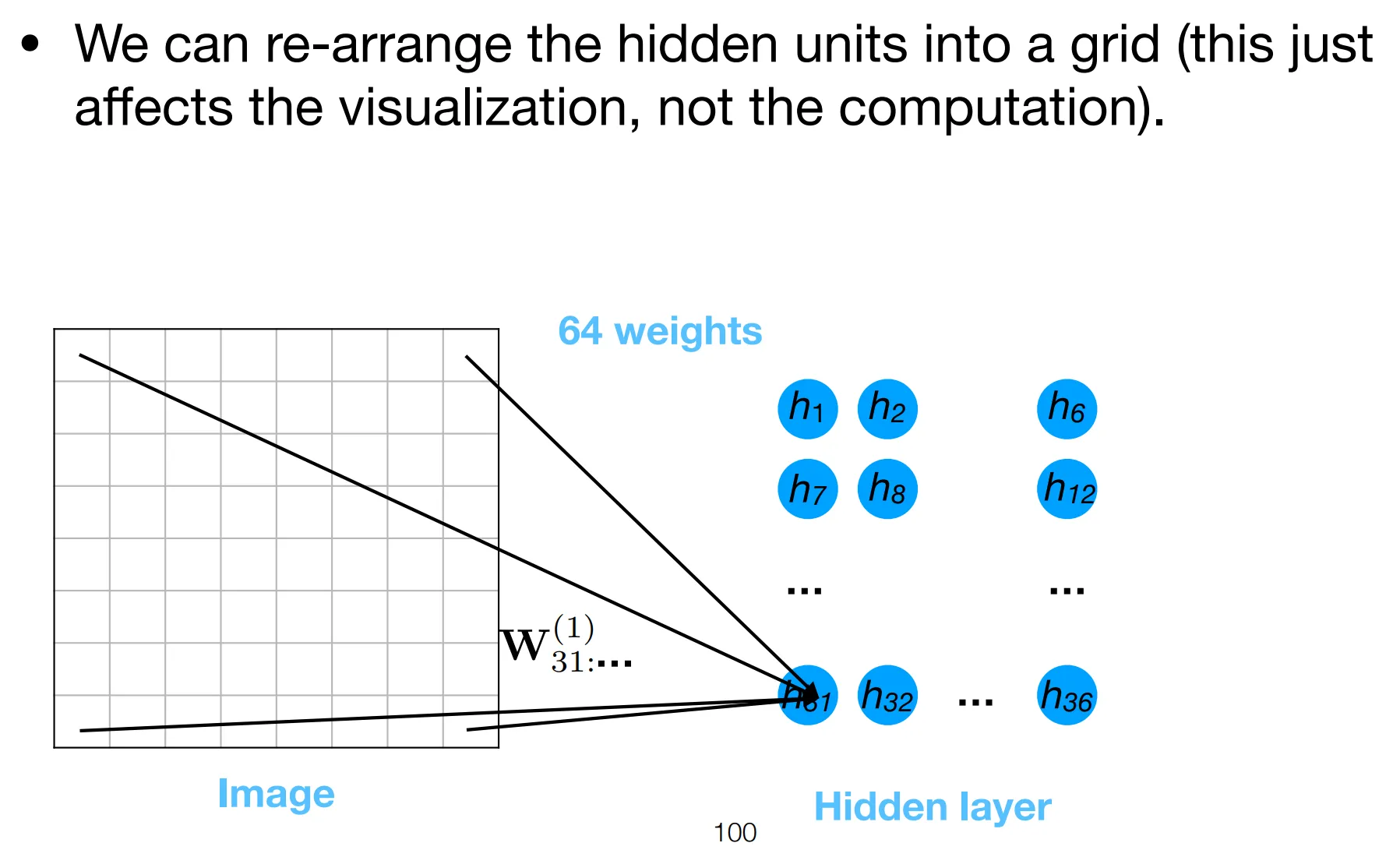
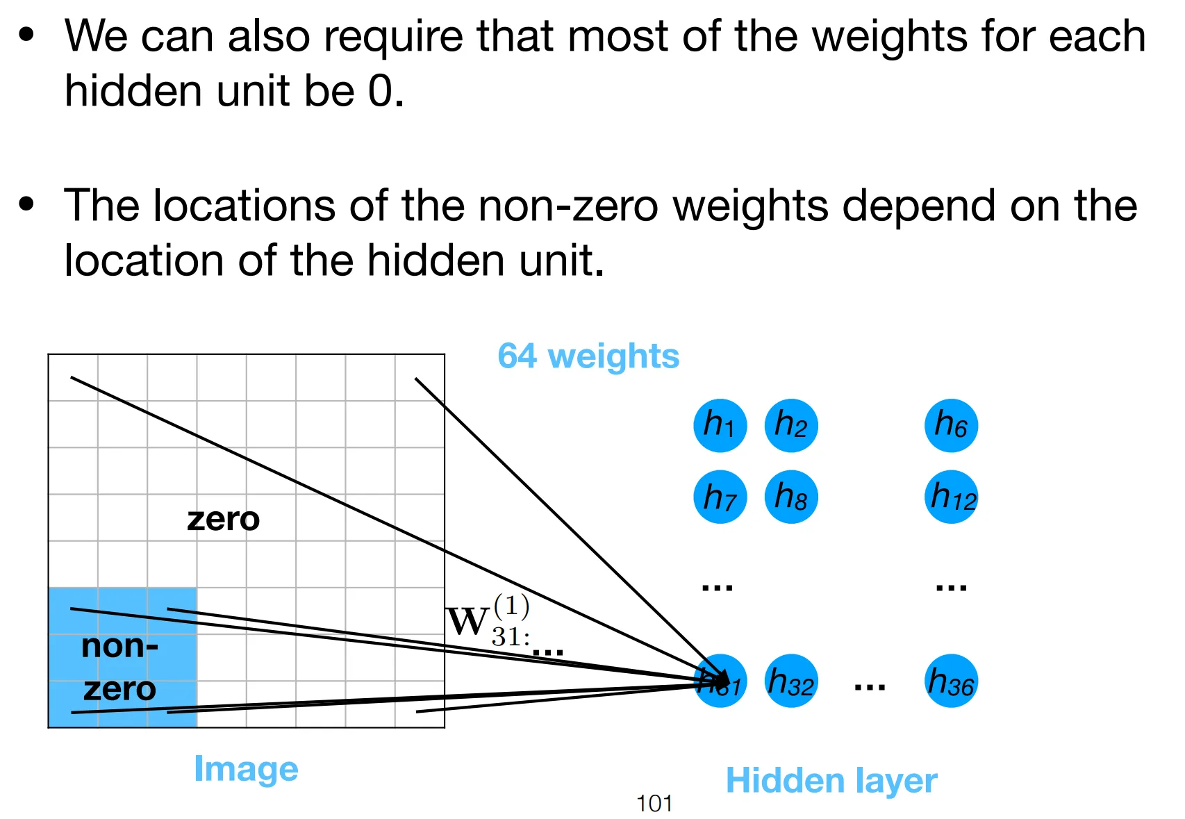
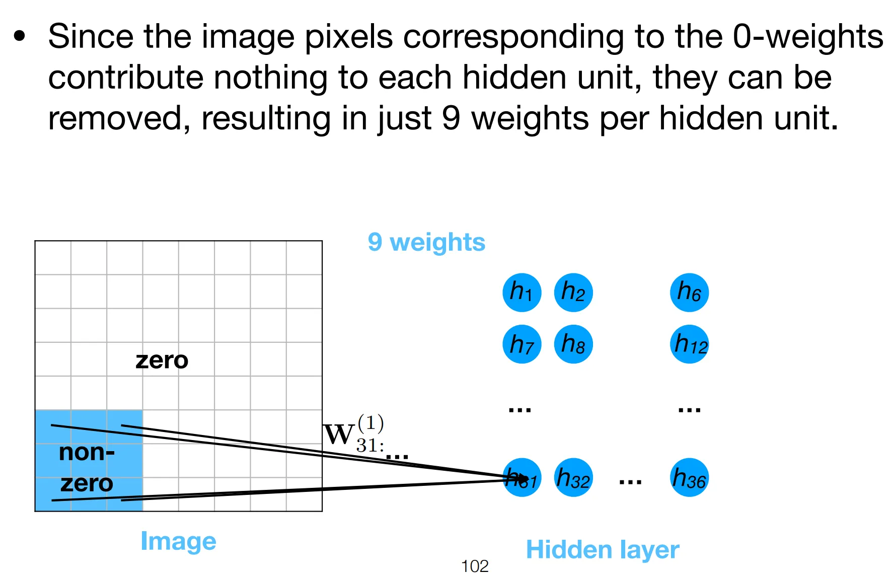
Essentially, we are restraining each neuron’s attention to a patch, local to its position.
- The position of neuron determines which patch it attends to.
- All neurons share the same filter parameters, forcing them to “agree on” the same features to detect.
Graph convolution networks (GCNs)
Section titled “Graph convolution networks (GCNs)”Representing graphs
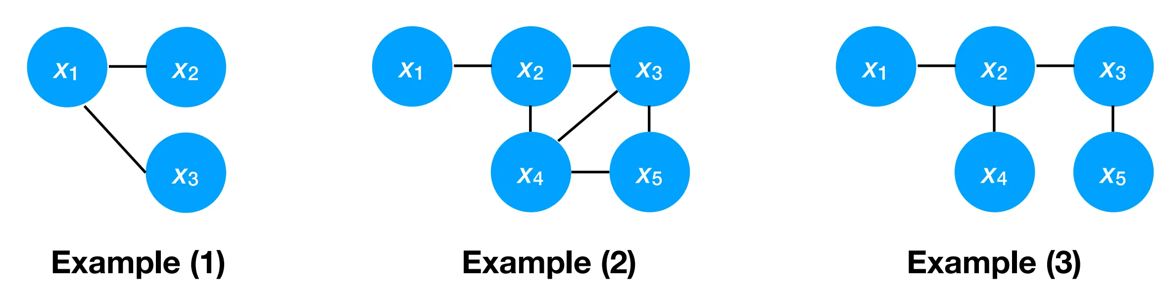
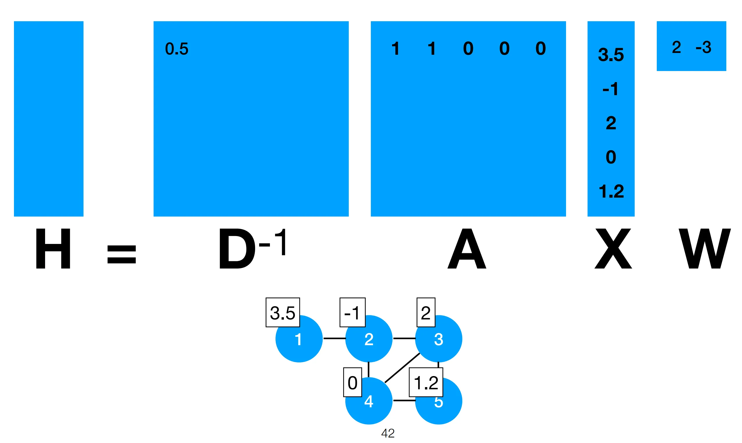
Section titled “Representing graphs”Starting from the classics, we represent each graph with an adjacency matrix (list of list of neighbors) and a degree matrix, a diagonal matrix that represents how many neighbors a node has (sum of the rows of adjacency matrix basically). We also annotate each node in the graph with a feature vector x_i.
For example:
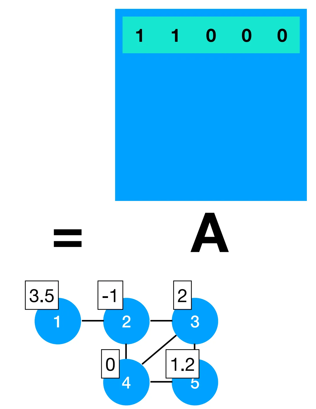
Then D[0] is just 2 since we also assume every node has a self-edge.
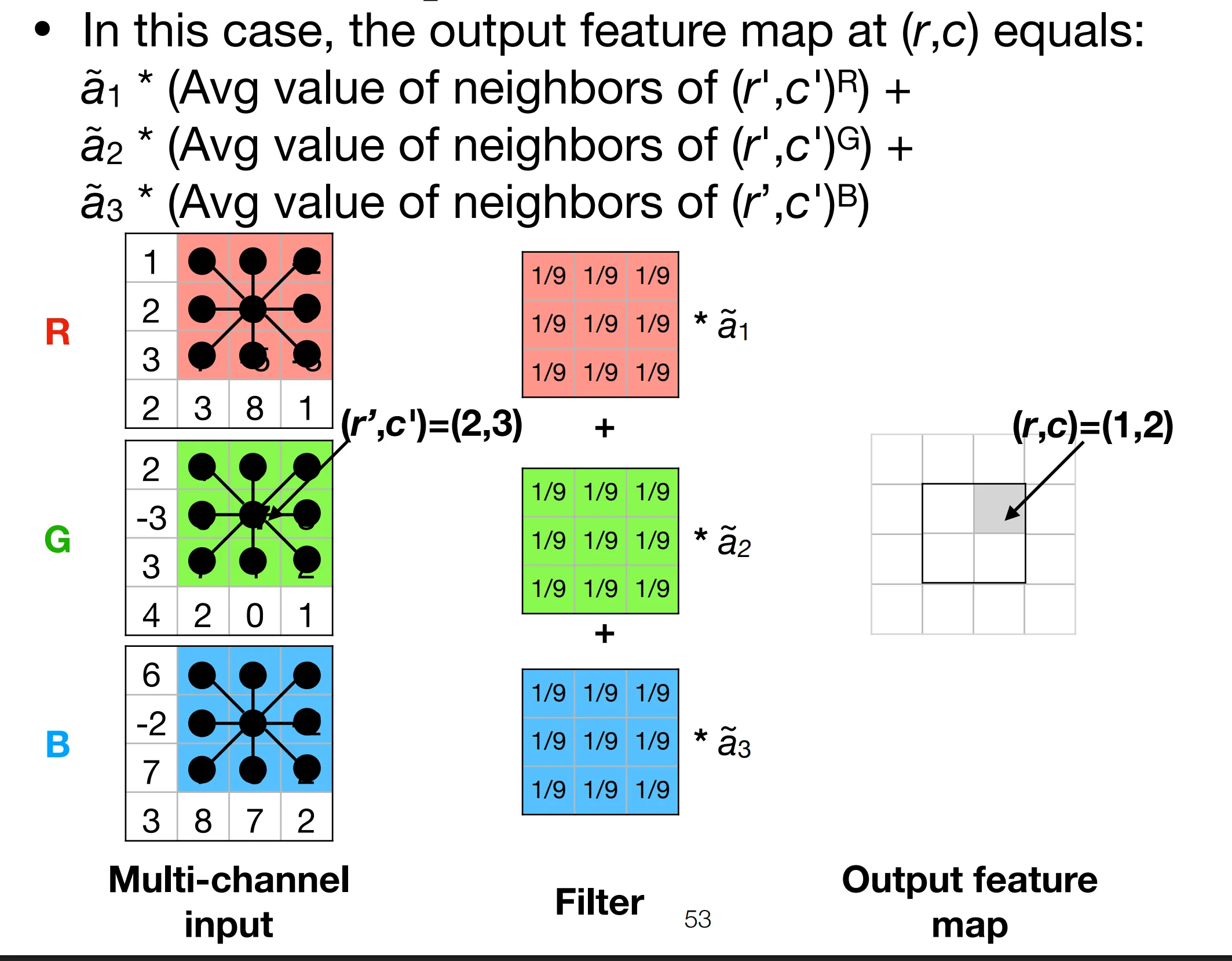
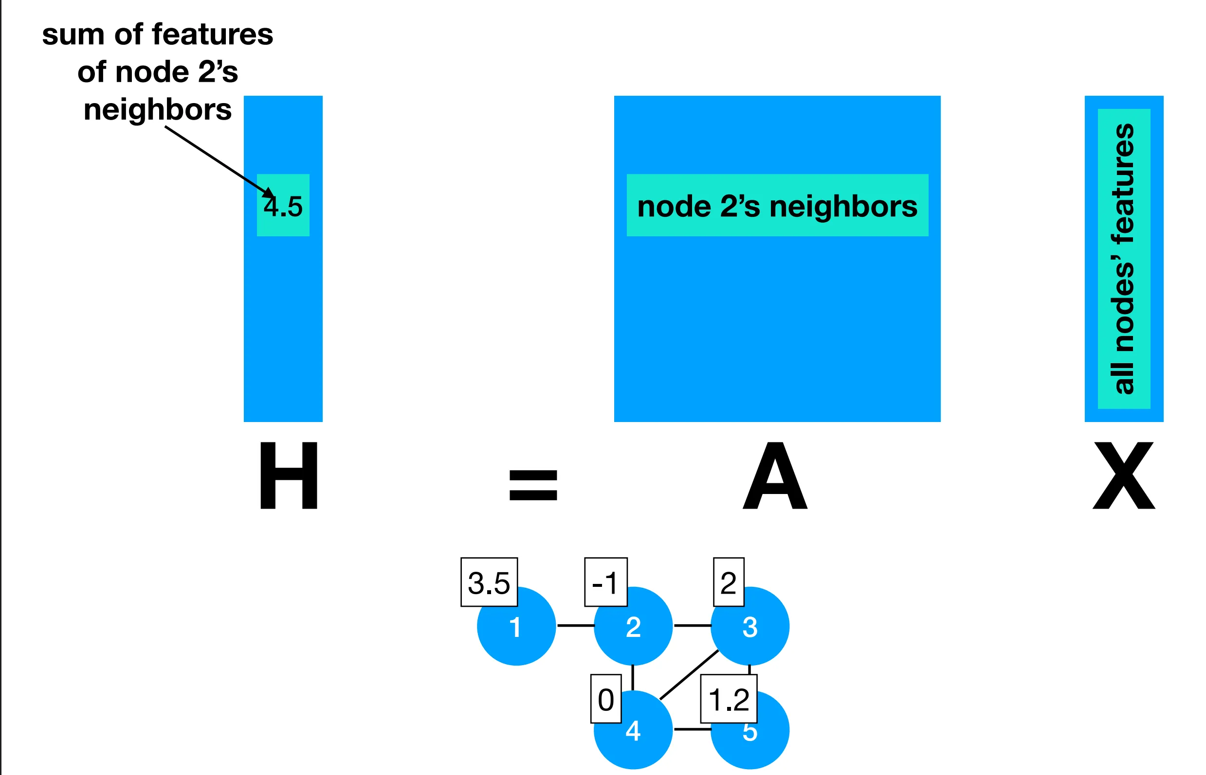
As a consequence, multiplying A and X gives us the sum of the features of a node neighbors, for every node in the graph, like so:
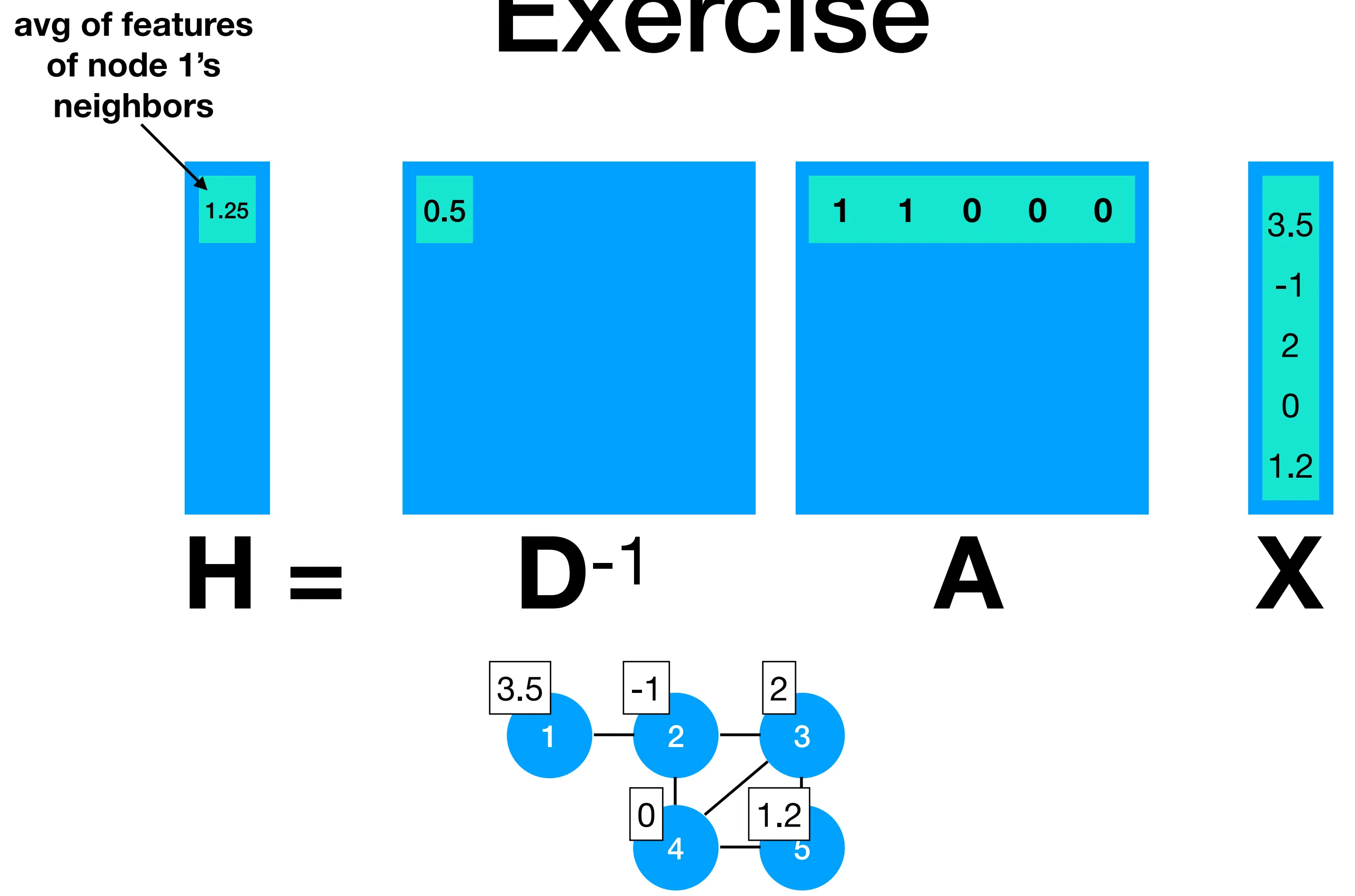
When dividing this by number of neighbors each node has (i.e., multiplying by the inverse of the degree matrix), we get the average of the features of a node’s neighbors (including itself):
Applications
Section titled “Applications”- Social networks (i.e., homophily, “birds of a feather flock together”, “people are the average of their friends”)
- Drug discovery: molecules are graphs of atoms, and we want to predict the binding affinity of a molecule to a particular receptor.
Flaw of classic neural networks
Section titled “Flaw of classic neural networks”In a neural network that processes tensors, the input is always of fixed size and topology (a vector of features of the same size, images of fixed size, etc.).
In contrast, a neural network that processes graphs should be able to process graphs of different sizes and topologies.
Not to say that they are all useless, we can borrow 2 things from CNNs to build graph convolution networks:
- An operation that summarizes the input no matter the input size: Pooling
- An operation that is applied the same at each position regardless of the input topology: Convolution
GraphConv
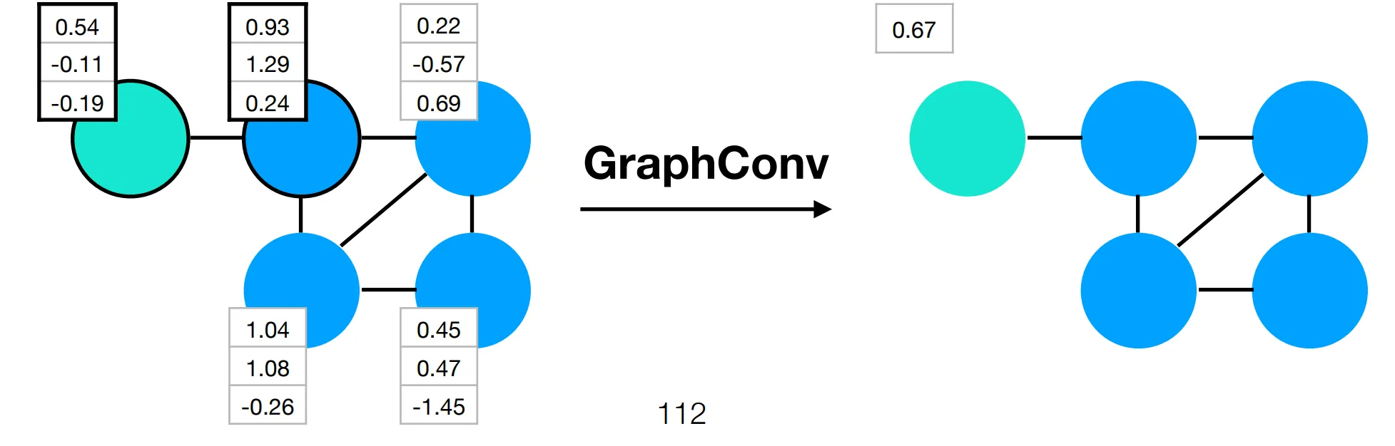
Section titled “GraphConv”In a GraphConv layer of a GCN, the feature vector at each node is transformed based on the feature vectors of neighboring nodes.
The size & topology of the output graph is the same as the input graph.
In contrast to image convolution:
- The convolution filter in a GCN has a variable size depending on the input location.
- There is no spatial ordering to the elements in the filter.
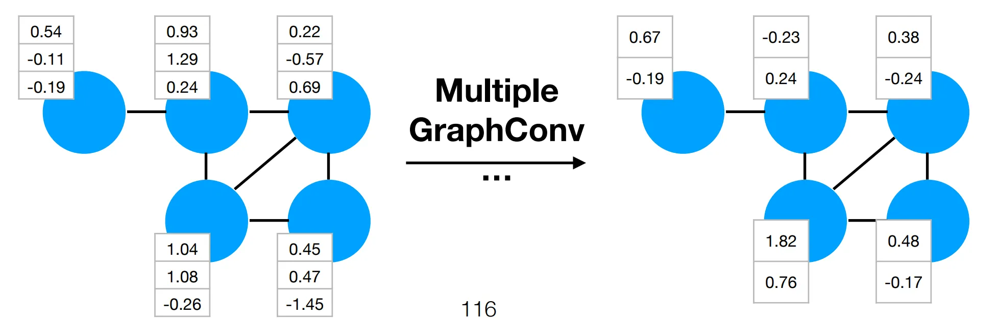
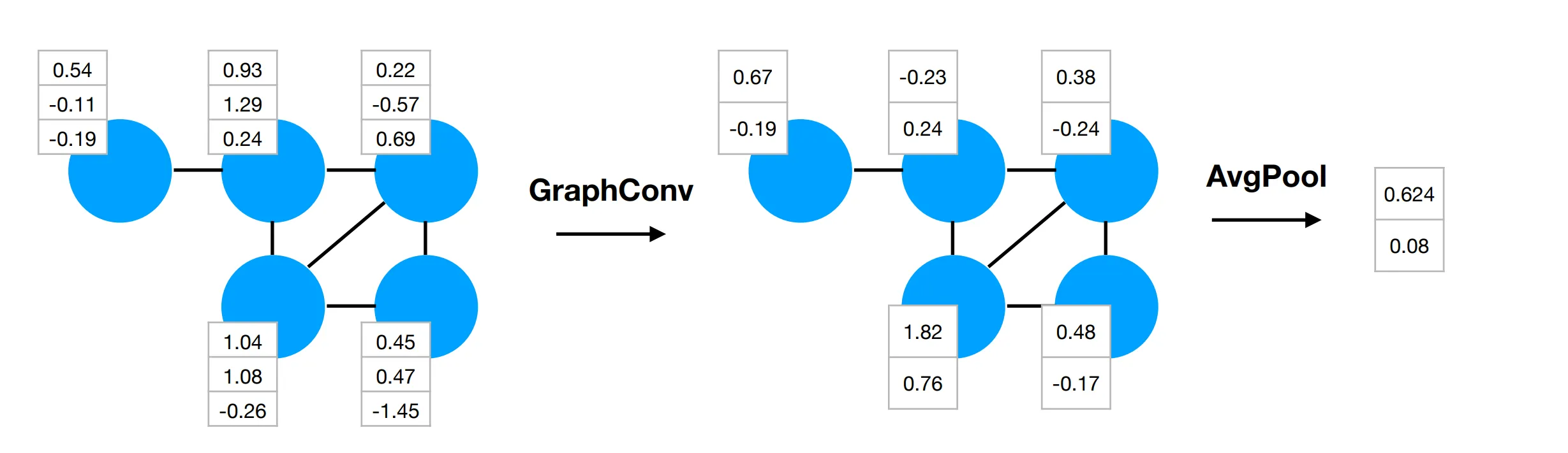
GCNs often consist of multiple GraphConv layers followed by a pooling layer (to perform final classification), e.g.:
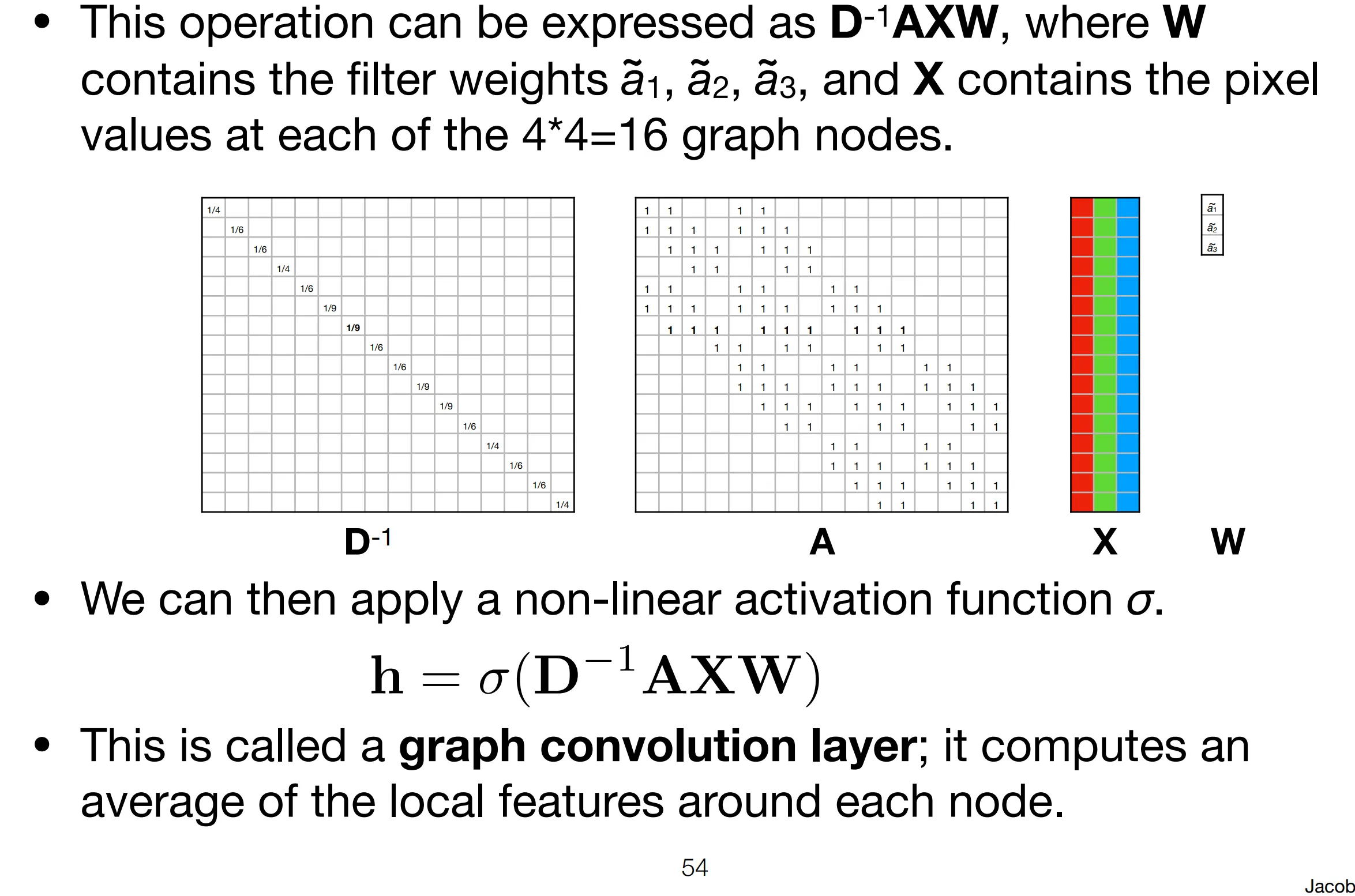
By adding a weight matrix W to the convolution step above before multiplying by the adjacency matrix, we map from m to k dimensions, where m is the size of the input feature vector and k is the size of the output feature vector. This is just a FC layer.
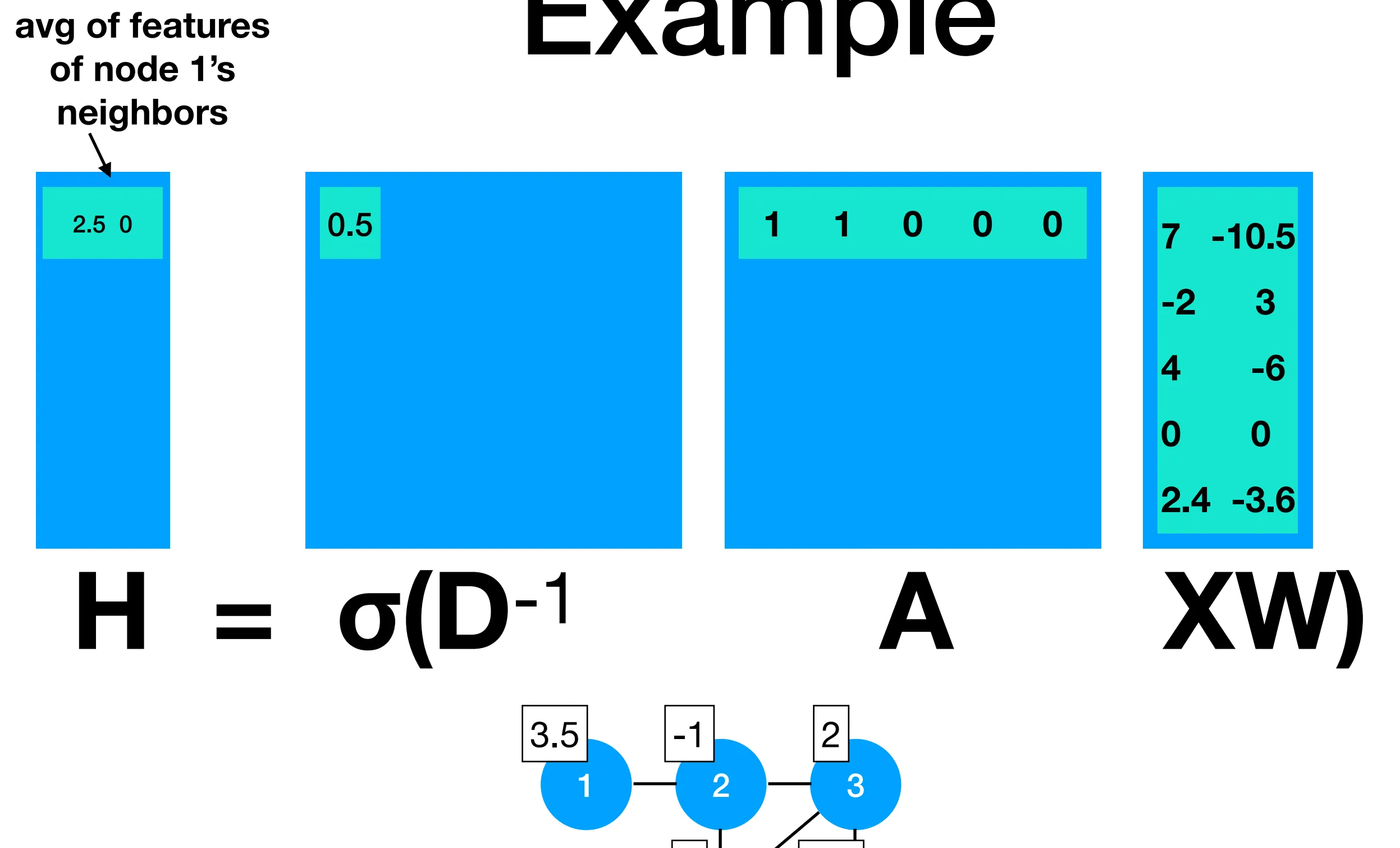
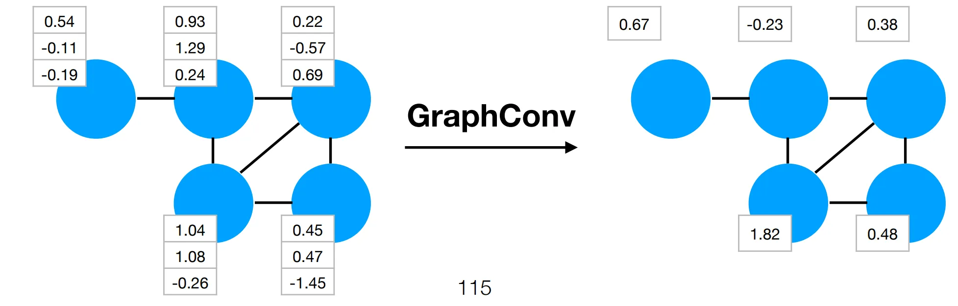
So a GraphConv layer maps each node’s feature vector to a new space (either up or down in terms of dimension) then assign each node the average of itself and its neighbors’ new features. Lastly, a nonlineary is applied.
A GraphConv layer computes an average of the local features around each node.
Intuition: notice how a GraphConv shares the same parameters across all nodes, just like how a CNN shares the same parameters across all pixels. This is a strong form of regularization like CNNs. Since the filter size is variable and unstructured, so the model has to learn to detect features that are useful across all possible filter sizes and topologies.
Properties of GraphConv
Section titled “Properties of GraphConv”CNNs are restricted GCNs
Section titled “CNNs are restricted GCNs”On images, this function still performs 3-d convolution. However, it’s “restricted” in the sense that all filter elements are constant within each channel.
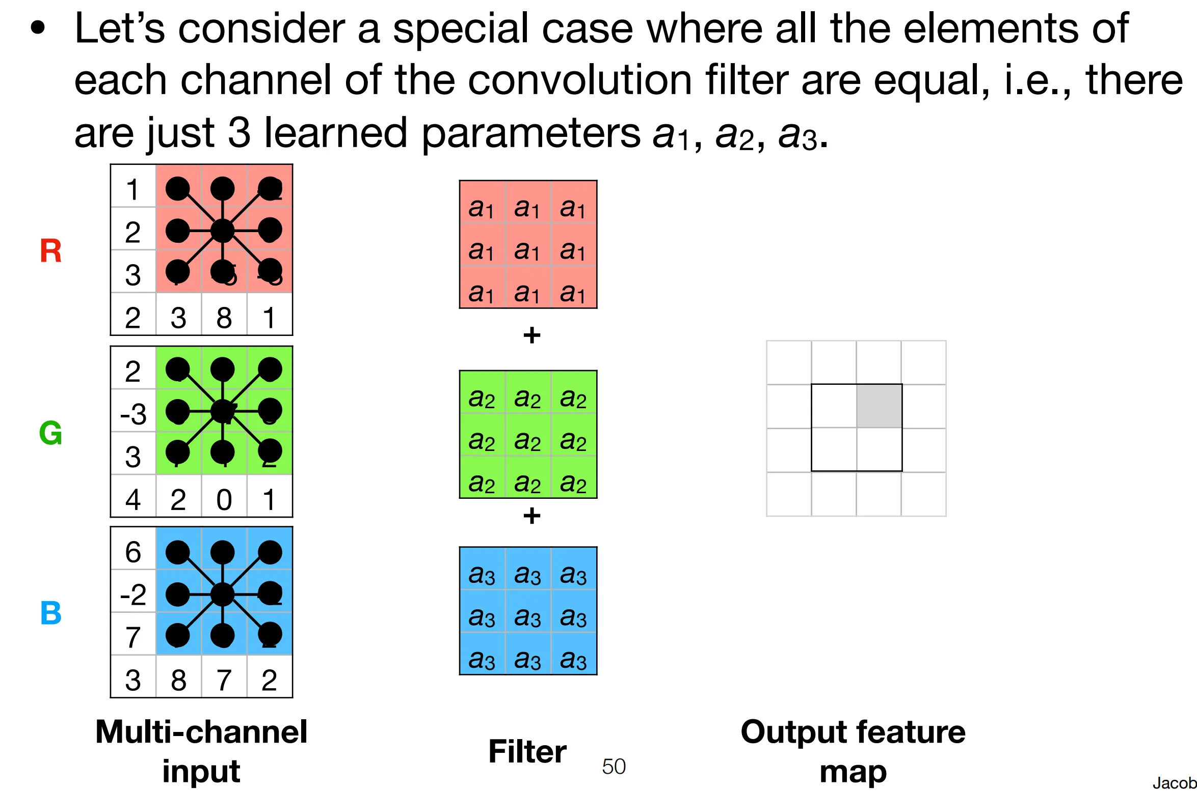
After reparameterizing: