Entropy in deep learning

Thesis: prediction = compression = intelligence

In other words, you could think of LLM pre-training instead of predicting the next token, it’s creating the most efficient text compressor.

Motivating example: sending instructions using a bitstream

The constraint: No code word can be a prefix of another one. This is called the prefix condition. Codes that satisfy the prefix condition are called prefix(-free) codes.

The trade-off: You could encode the most common instruction with fewer bits, but then all possible code words that start with that code word are not available for encoding other instructions. This is the trade-off between the length of the code word and the number of code words available.

The insight: The optimal code is the one that minimizes the expected code word length, which is , where is the probability of the instruction and is the length of the code word for that instruction. This happens when the code word length is proportional to the negative logarithm of the probability of the instruction, i.e. . How do we prove this?

Tip

Another way to read is how many times do you chop the possibility space in half until you get to the instruction.

What is the lower bound on the expected code word length?

Random noise should be incompressible. Therefore, a perfect compressor should produce a bitstream that is indistinguishable from random noise.

Let X be a random variable representing a message chosen uniformly at random from the set of all possible binary strings of length . Because every message is equally likely, the probability of receiving any specific message is: .

Because each of the messages is equally likely, the probability of any single message occurring is . The information entropy of this source, which dictates the absolute minimum average number of bits needed to represent the data without loss, is calculated by summing the self-information across all outcomes: bits. According to Shannon’s theorem, the expected codeword length of any uniquely decodable code is bounded by this entropy, meaning . Substituting our calculated entropy into this inequality yields , proving mathematically that the expected codeword length for a perfectly random source must be at least bits, confirming that truly random noise cannot be compressed on average.

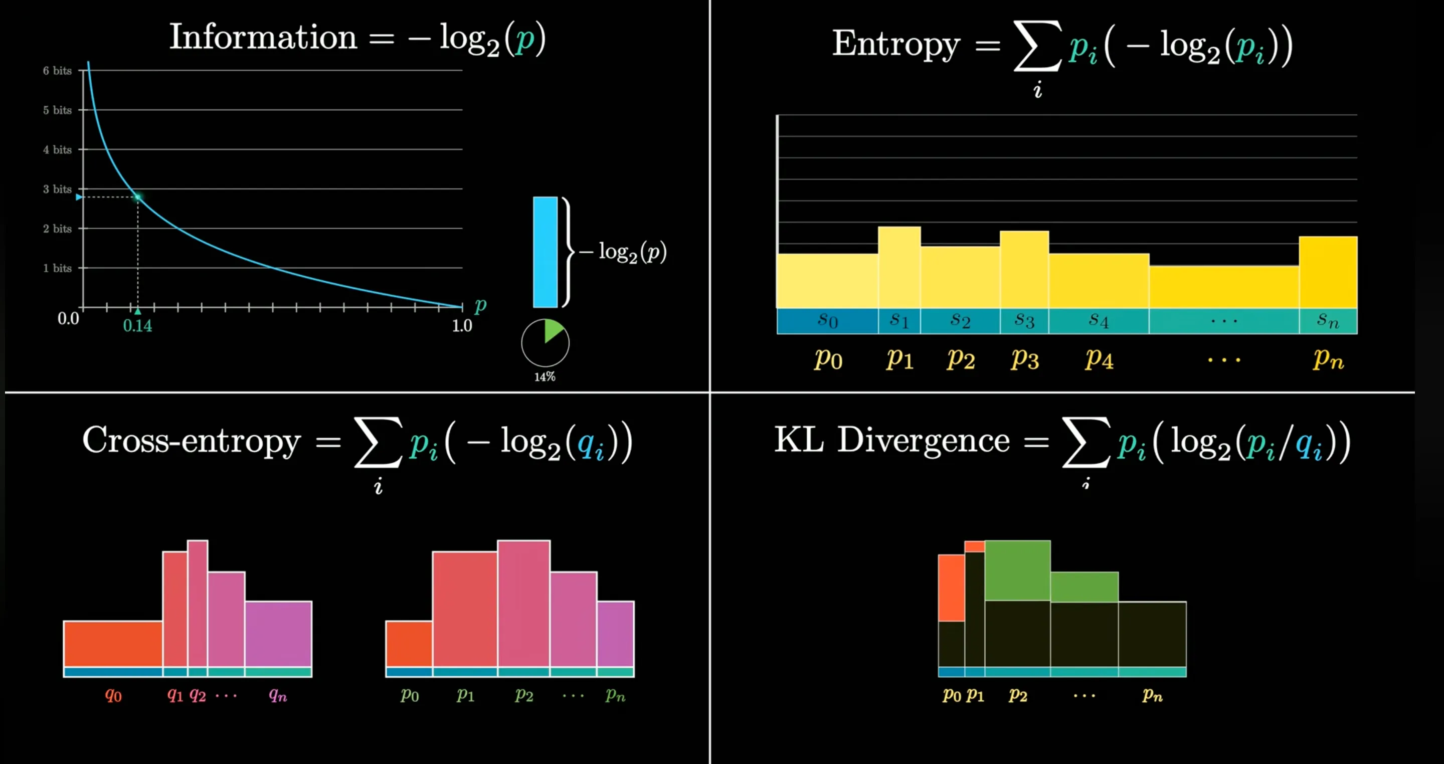
Information of an event

Same as the self-information of an event, which is defined as , where is the probability of the event. This means that the less likely an event is, the more information it carries when it occurs.

Entropy of a distribution

The entropy of a distribution is the expected value of the self-information of the events in the distribution. It is defined as , where is the probability of the event in the distribution. This means that the more uncertain a distribution is, the higher its entropy.

Caution

A uniform distribution is surprisingly, the most uncertain distribution i.e., high entropy because it represents maximum uncertainty and maximum possible choices.

Cross-entropy

Cross-entropy is how many bits on average you need to encode data from a distribution using a code optimized for a different distribution . It is defined as , where is the probability of the event in the true distribution and is the probability of the event in the model distribution .

Relationship to negative log-likelihood

They are the same in the context of a classification problem. Suppose:

• is the one-hot encoded vector of the label with the correct label at position
• is our predicted probabilities vector

In this setup, cross-entropy simplifies to:

However, similar to the overflow problem of naive softmax on real hardware, log softmax risks taking . We have to resort to the log-sum-exp trick:

KL divergence

KL divergence is the difference between the cross-entropy and the entropy of a distribution. It is defined as , where is the probability of the event in the true distribution and is the probability of the event in the model distribution . KL divergence is a measure of how much information is lost when using the model distribution to approximate the true distribution .

KL divergence is not a distance by definition, since it is asymmetric and does not satisfy the triangle inequality.

The reason it is non-negative is that entropy is the minimum achievable expected code length for a source distributed according to . Since no coding strategy can outperform the optimal code for the true distribution , we necessarily have

Therefore

In other words, the probability distribution (our model) cannot yield a lower expected encoding cost than the true distribution , because already represents the theoretical lower bound on the expected code length for data generated from .

Recap