Robot control & MDPs

Robot control

Mathematical representation of robot motion

Robots come in a wide variety of morphologies. How can we control them? We assume robots are rigid bodies and robot motion can be represented as rigid-body motion. Rigid body means that any two points on the robot maintain a constant distance. As such, we only have to track one point on the robot instead of multiple.

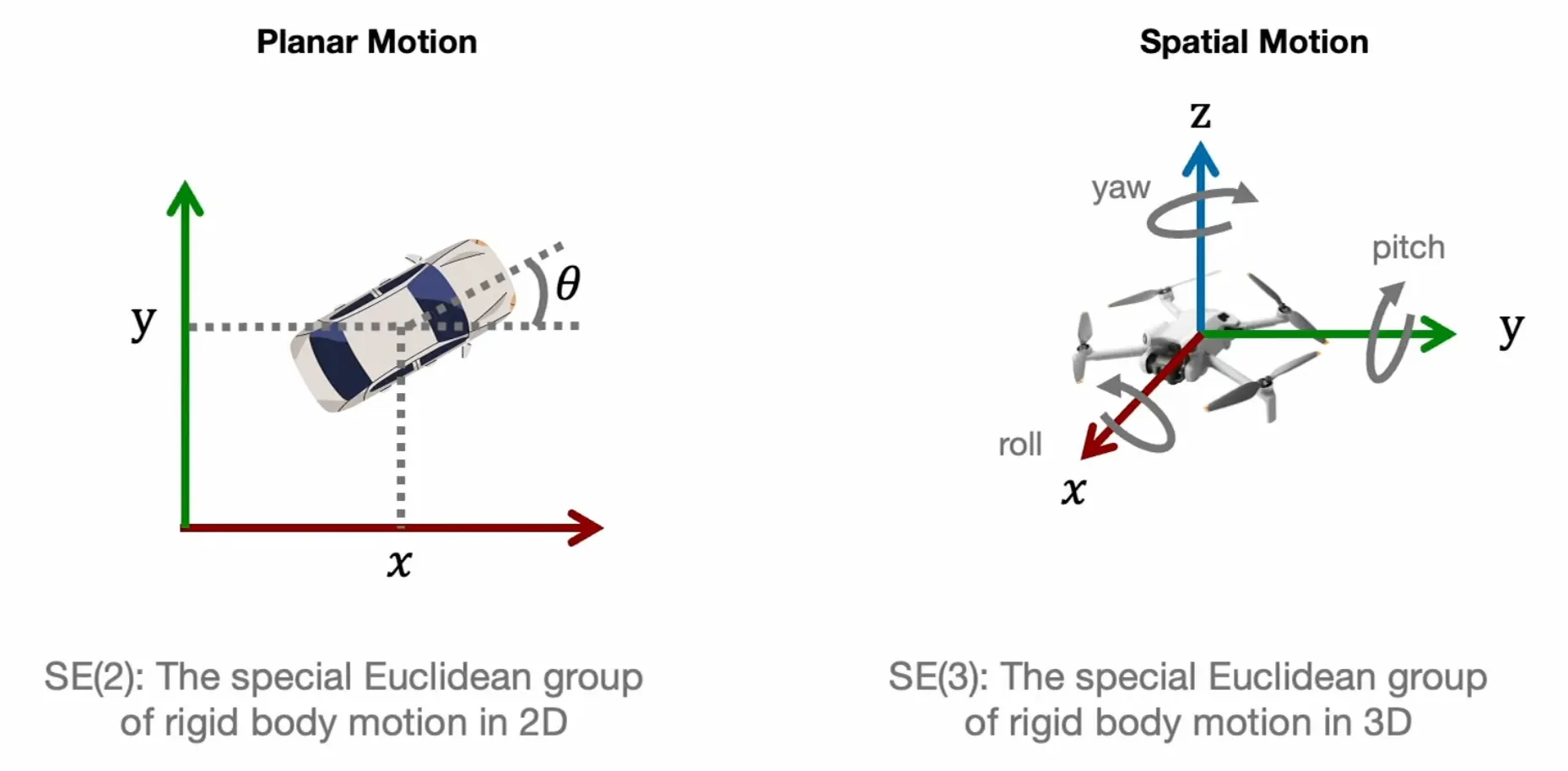
To represent robot motion mathematically or in code, we use homogeneous transformation matrices.

SE(2): 3 degrees of freedom

SE(3): 6 degrees of freedom

In order for these to be valid rotation matrices, they must satisfy the following properties:

1. The matrices must be orthogonal, meaning that the transpose of the matrix is equal to its inverse.
2. The determinant of the rotation matrix must be equal to 1, which ensures that it represents a proper rotation without any scaling or reflection.

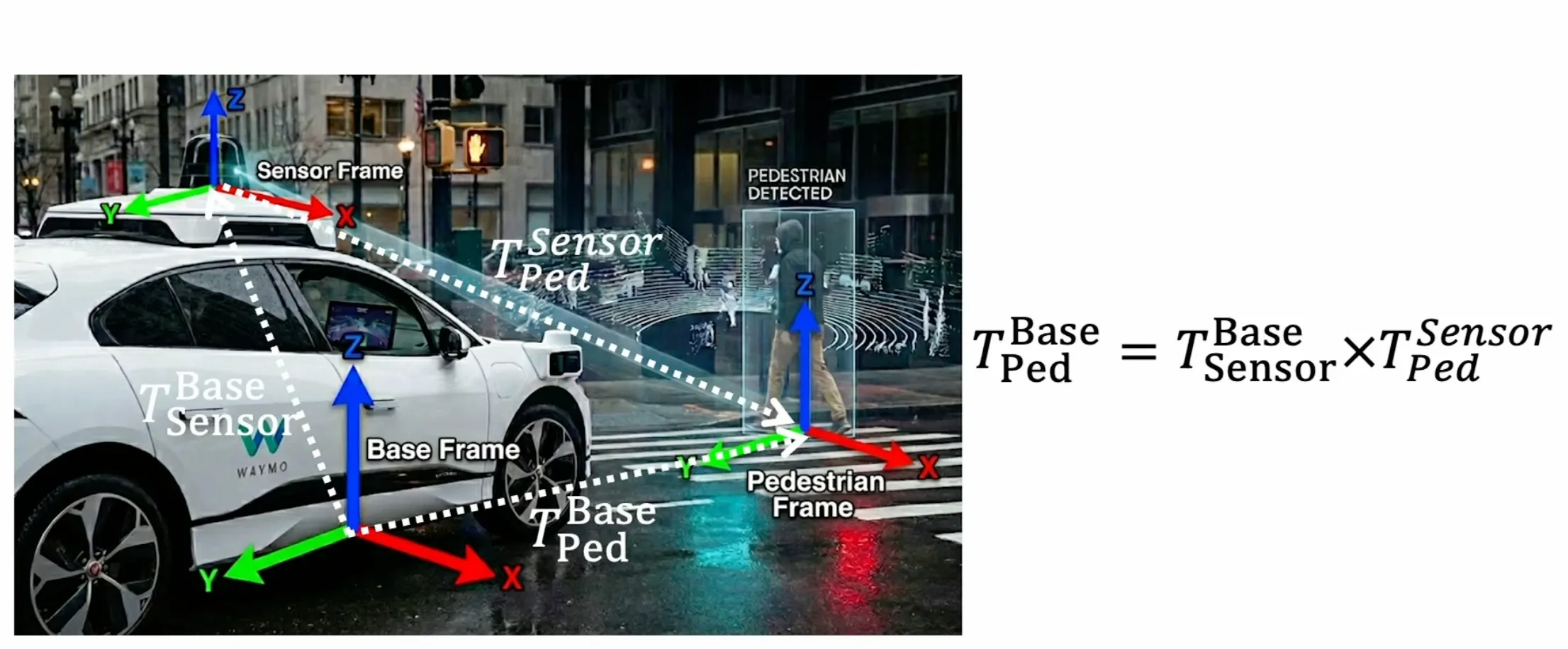
Why do we care about these rotation matrices? It’s so that we can chain transformations together to determine an object’s position in the base frame given its position in some sensor’s frame.

Note

To determine , you would typically perform sensor calibration.

Note

Inverting a rigid body transform

A transform has two parts: rotation and translation . The inverse is:

So to go from :

To transform any world-frame point into the base frame:

Intuition: translate so the base is the origin, then rotate into the base’s orientation.

Key intuition: “undoes” the rotation applies. If rotated from base world, then rotates from world base.

Robot embodiment

However, robot is not a single solid body. Most humanoids have links (rigid parts) that are connected by joints (which allow for relative motion between the links), and end effectors (which are the parts of the robot that interact with the environment, such as hands or grippers). To find out the position of the end effector in the base frame, we can apply the transform chaining technique above.

For robot arms, Franka is a typical example of a 7 degree of freedom robot arm.

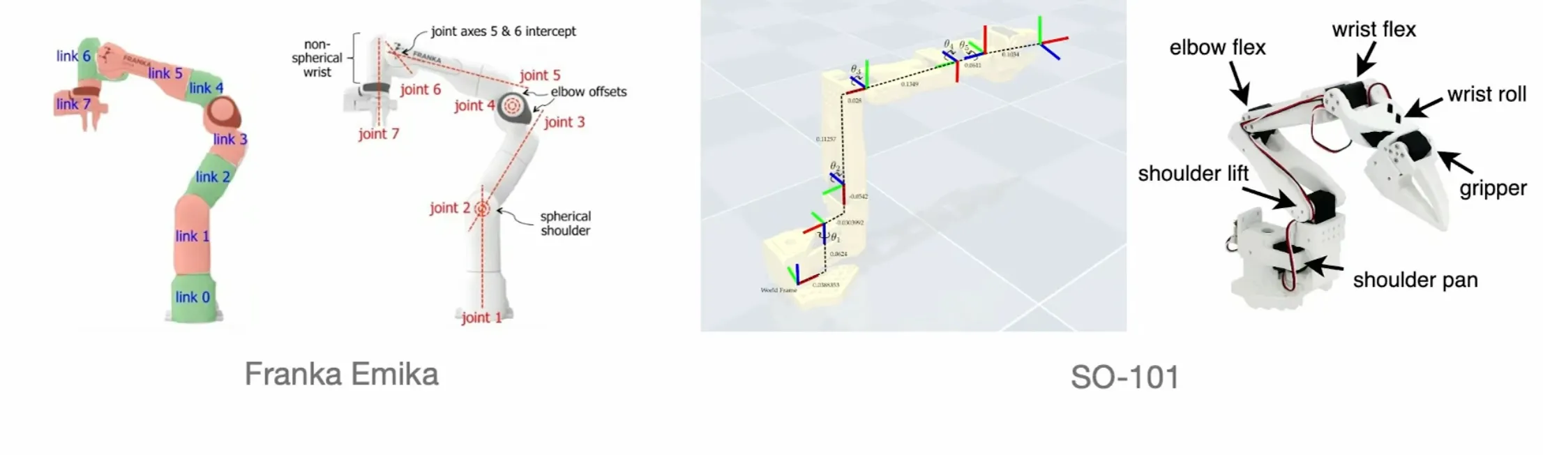
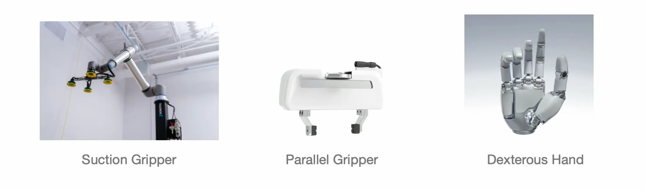
For effectors, suction grippers, parallel grippers, and dexterous hands are common types.

Hard-coded geometry vs learned representations

Intuition: Motion planning in C-space quickly becomes intractable as the number of degrees of freedom increases. In modern robot learning, we don’t want to have perfect world information, we want to learn a policy that can learn to feel where the obstacles are implicitly and recognizing automatically invalid states.

Task space: the manifold in which the robot’s task is naturally defined, independent of its embodiment. If task space dimension is less than the robot’s degree of freedom, then the robot is redundant. If task space dimension is greater than the robot’s degree of freedom, then the robot is underactuated.

Example: task is whiteboard cleaning, task space is whiteboard surface .

Example: Franka’s arm C-space, workspace, and task space

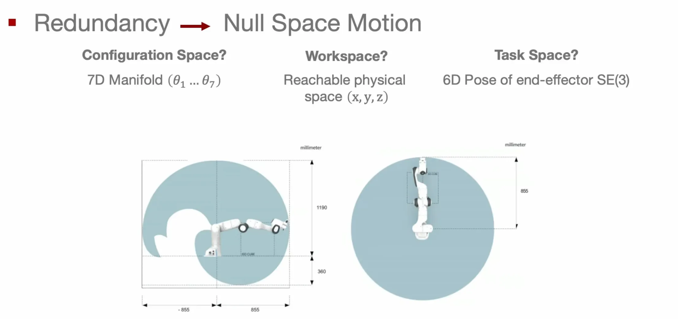
Example of redundancy leading to null space motion: a Franka arm holding a cup of coffee can move its elbow without affecting the position of the cup. This is called null space motion, and it can be used to optimize for secondary objectives such as avoiding obstacles or minimizing energy consumption.

Forward and inverse kinematics

Forward kinematics: given the robot’s joint angles, compute the position of the end effector in the base frame. This process is straightforward and can be done by chaining together the transformations from the base frame to the end effector frame.

• Maps from C-space to task space,
• Deterministic, but not bijective (multiple joint configurations can lead to the same end effector position).

Inverse kinematics: given the desired position of the end effector in the base frame, compute the joint angles that will achieve that position. This is much harder as there might be multiple configurations to achieve the same end effector pose.

• , mapping
• Often non-unique or has no analytical solution
• Optimization-based inverse kinematics (IKs): introduce cost function (how far away current end effector pose is from target pose), add some secondary constraint (obstacle, energy), and optimize for the joint angles that minimize cost with gradient descent.

Optimization-based inverse kinematics

Objective: Minimize the distance between the current end effector pose and the target pose.

Loss:

Update:

Gradient of the loss w.r.t. the joint angles:

where is the Jacobian matrix of the forward kinematics function with respect to the joint angles .

Jacobian method:

Note

You can think of this Jacobian matrix as how much each individual joint affect the end effector 6D pose (x, y, z, roll, pitch, yaw) and has shape 6 x num_joints.

Note

Deriving the gradient of the loss:

Damped least squares

The problem: Near a singularity, the Jacobian loses rank and the simple update can blow up with enormous joint velocities. To avoid this, we add a damped term to the update.

Plain gradient descent uses as a rough stand-in for . DLS derives a better update by solving an explicit optimization over . The idea: find the joint velocity such that , but also penalize large :

Take derivative w.r.t. and set to zero:

Caution

Why the code uses a different but equivalent form?

The above requires inverting an matrix. For a 7-DOF arm, that’s . But there’s a matrix identity (provable via Woodbury):

So equivalently:

When (task space smaller than joint space, which is the common case — 6D pose vs 7 joints on a Franka), the second form is cheaper. This is exactly what the code does:

A = J @ J.T + damping * np.identity(6)   # 6×6, not n×n
scaled_err = np.linalg.solve(A, weighted_err)  # solve 6×6 system
qdot = J.T @ scaled_err                        # n×1 update

So the full lineage is: loss function → gradient → DLS regularization → equivalent small-matrix form → numerically stable solve instead of explicit inverse.

The connection to the lecture: the lecture’s gradient is actually a special case. As , DLS approaches the Moore-Penrose pseudoinverse , which gives the minimum-norm joint velocity that achieves the desired end-effector motion. The lecture’s is a looser, cheaper approximation of the same thing — it points in roughly the right direction but doesn’t scale properly with the Jacobian’s geometry. The damping gives you a knob: higher → more stable near singularities but slower convergence; lower → closer to the true pseudoinverse but can go unstable.

Waypoint generation and following

IK only gives the target joints, but robot cannot jump there. To convert IK to motor commands, we need to take into account the time of movement. For this, we generate tiny waypoints along the path so the robot can follow them.

LERP

• Inputs: , time , and control frequency
• Number of waypoints: (one waypoint = one movement command)
• Normalized time progress:
• Waypoints:

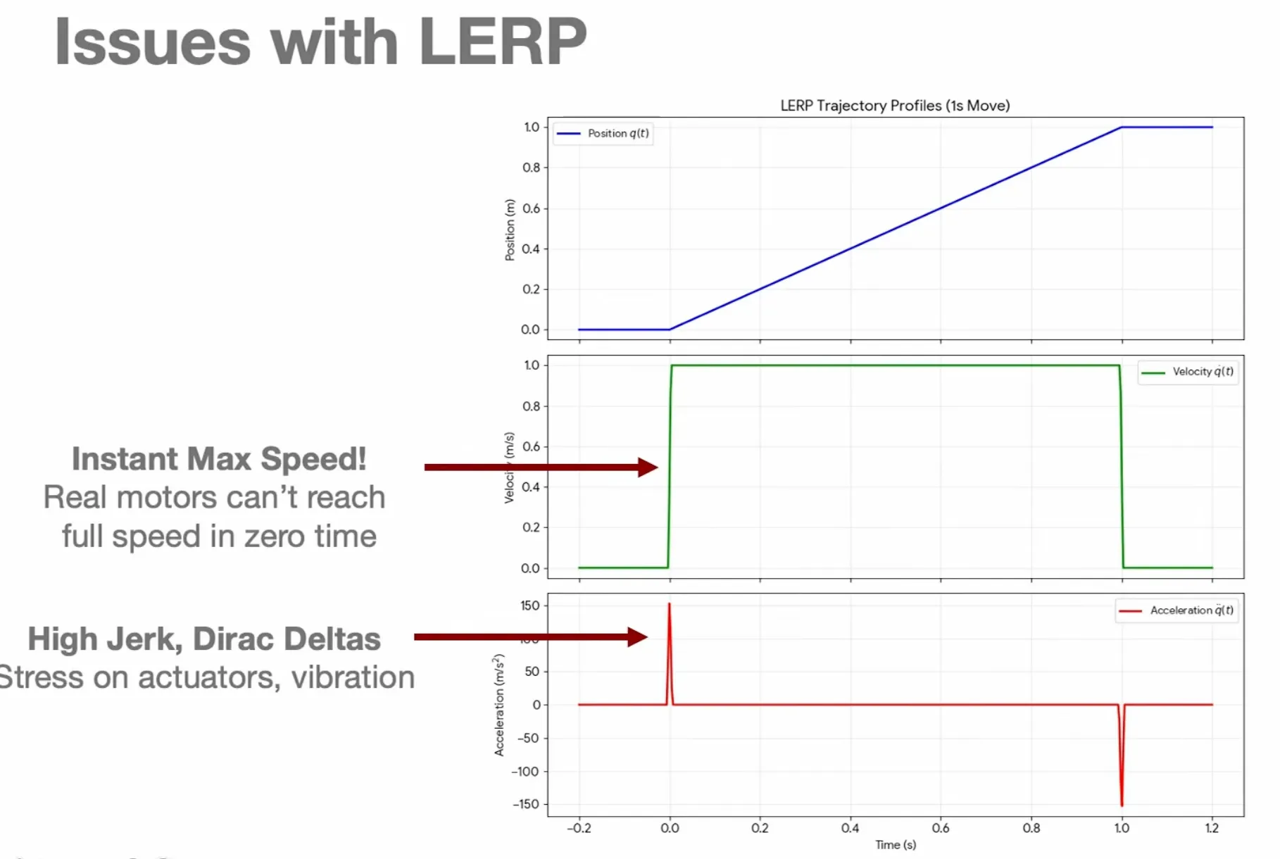
However, many issues with LERP:

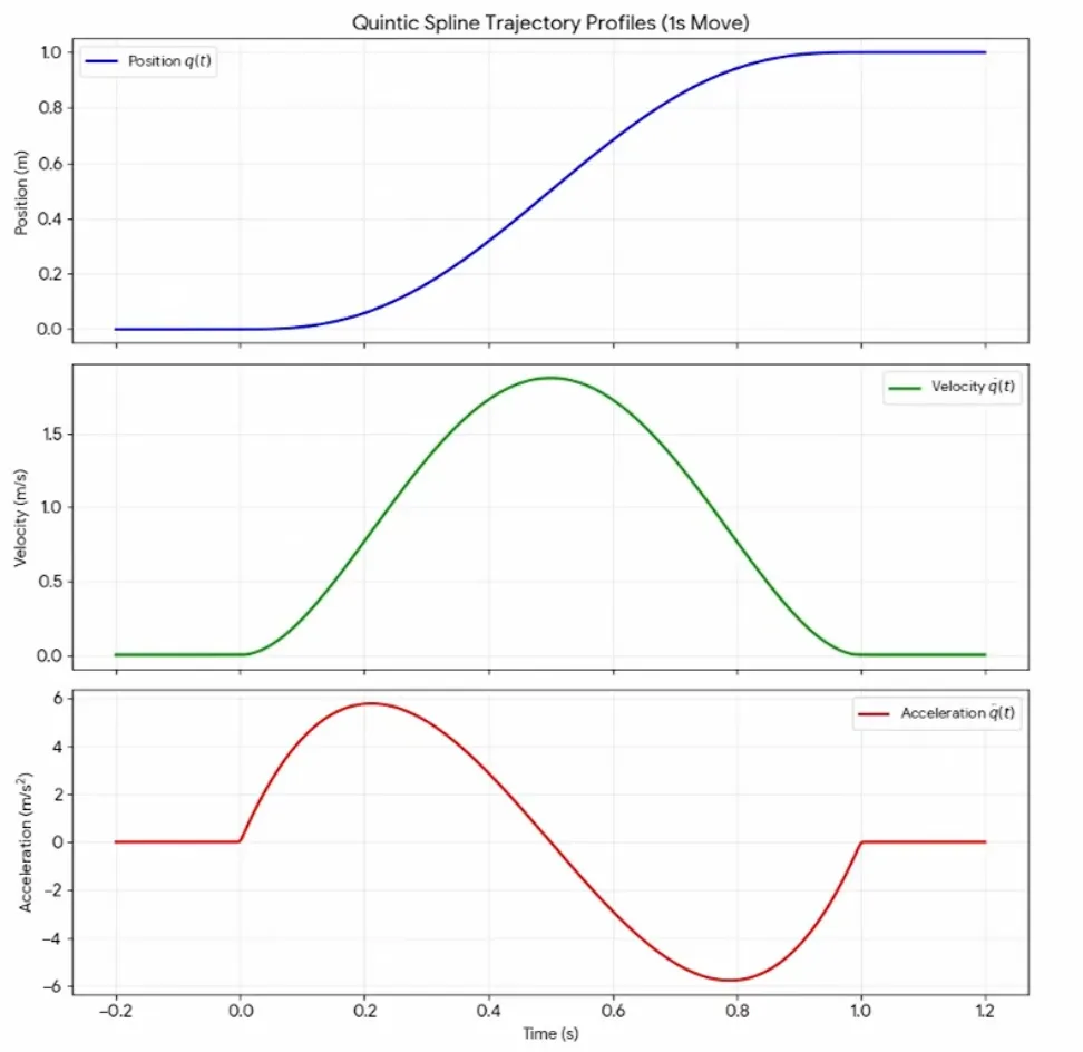
Quintic splines

Thus, most controllers use quintic splines, a polynomial-based method, to generate waypoints, i.e., representing the trajectory of each joint as a 5th order polynomial.

• Then add 6x boundary conditions for smoothness:
  • Start and end with no velocity and acceleration, while keeping position
• Quintic time scaling:
• Standard for industry robots like Frankas

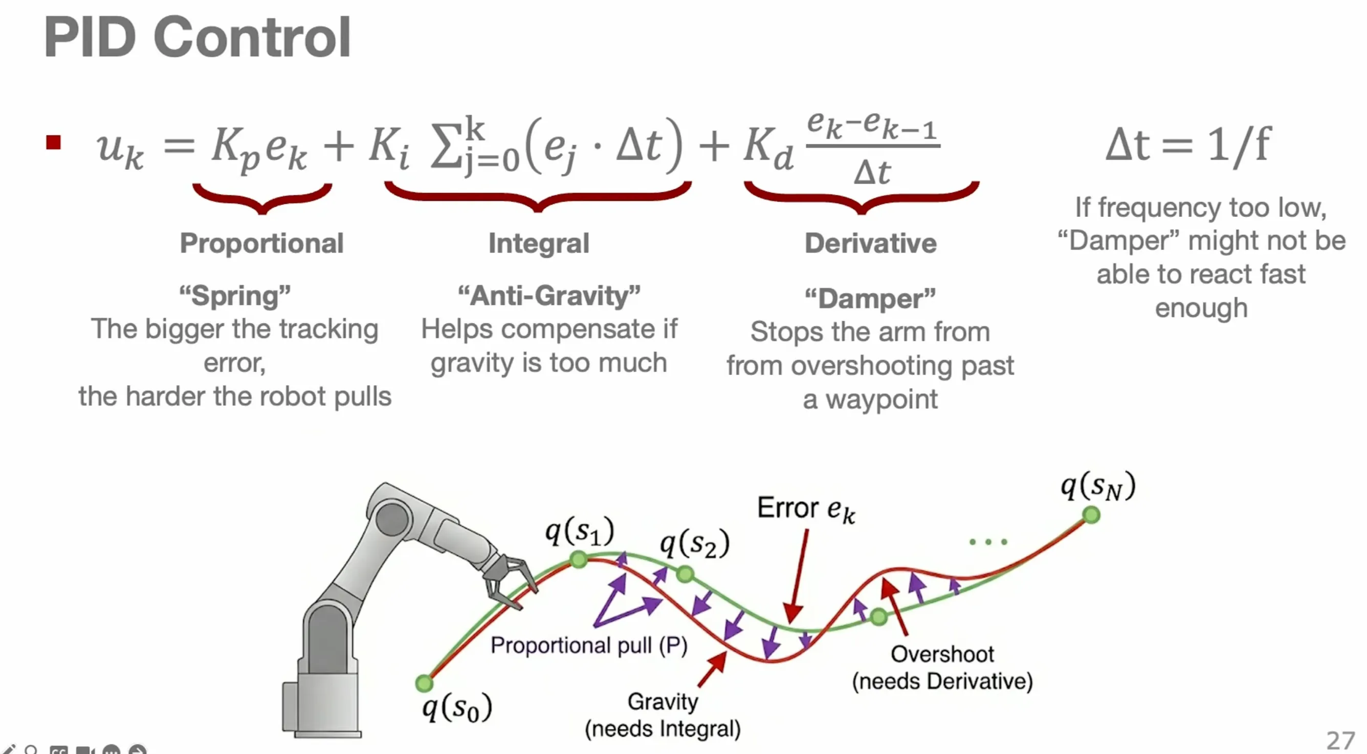
PID control

In the real world, the robot would not follow these waypoints perfectly because of friction and air resistance. Thus, we need to use PID controllers. The difference between the desired joint angles and the current joint angles (the tracking error) is fed into a PID controller. The controller calculates the appropriate control signal.

Given trajectory waypoints and current measurement, continuously calculate corrective motor commands ().

Tracking error:

Continuous form:

Discrete form:

Markov decision processes (MDPs)

Representing a policy

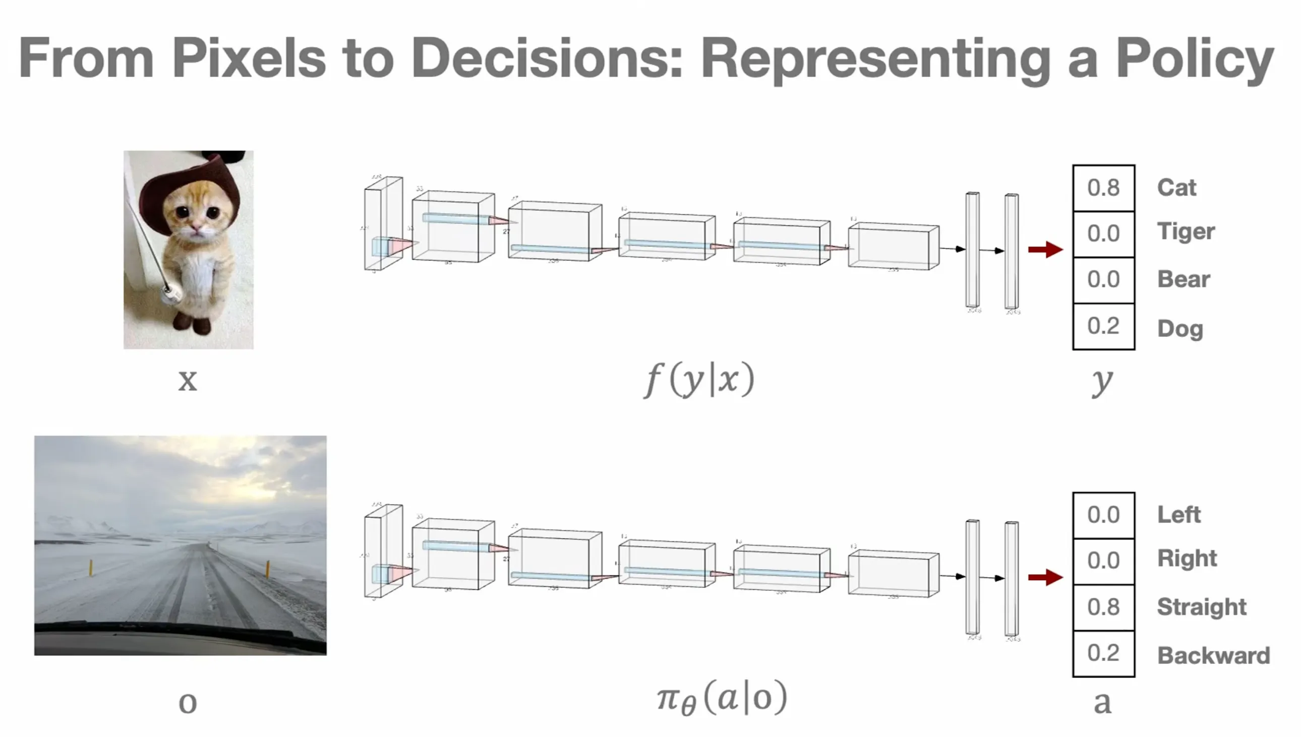
Not too different from an image classifier, the policy takes in an observation and outputs an action conditioned on the observation and outputs a distribution over actions.

Some environments are only partially observable, so (state, fully observable) becomes (observation, partially observable). is the action taken at time , and is the policy, which is a conditional probability distribution over actions given the observation, parameterized by the neural network weights, .

Markov property

Note

The Markov property for a system is satisfied when the next state of a system only depends on the current state and action, and not on any previous states or actions. In other words, the transition dynamics of the system can be fully described by the current state and action.

MDP

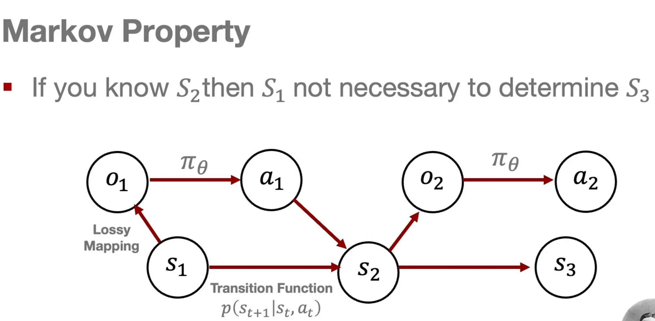
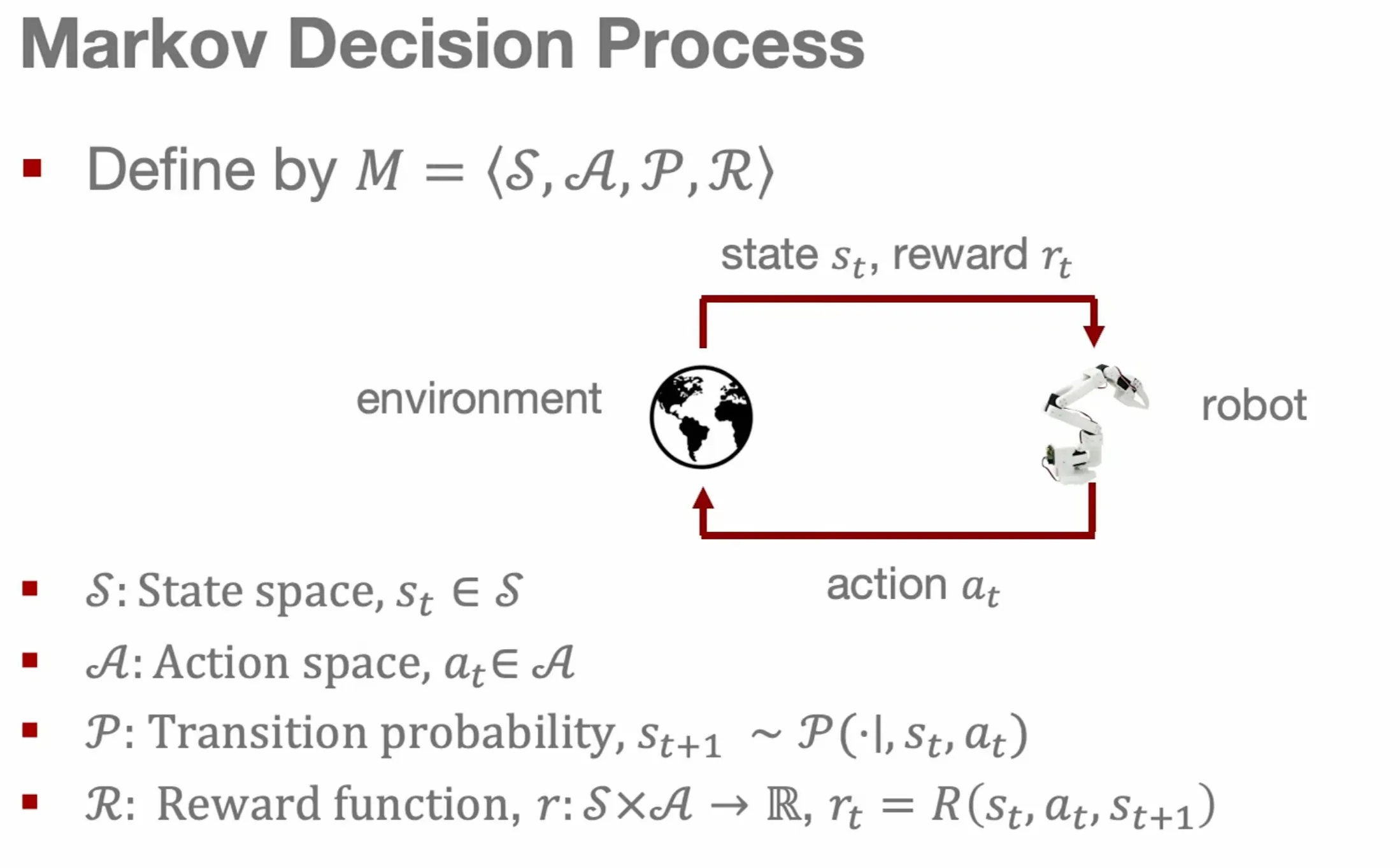
• State space can be discrete (chess, go) or continuous (robot movement)
• Similarly, action can be discrete (play a certain card from 64, keyboard WASD) or continuous (apply force in x, y, z direction)
• Transition model can be deterministic or stochastic . Uncertainty caused by sensor noise, motor overshooting, i.e., latent variables
• Reward function can be sparse (reward only at the end of the episode) or dense (reward at every step). E.g., robot arm trying to pick up a cup, reward only when it successfully picks up the cup (sparse), or reward based on how close the end effector is to the cup (dense).

Trajectory probability

How likely a trajectory is under a policy and transition model .

Caution

The transition dynamics and control policy are two different distributions that interact with each other. Not the same thing.

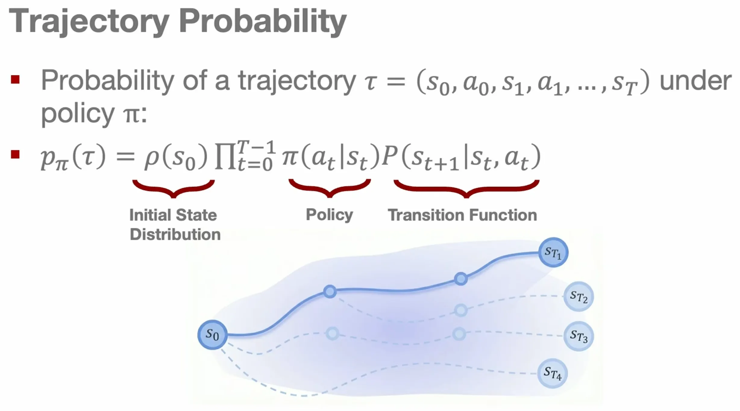
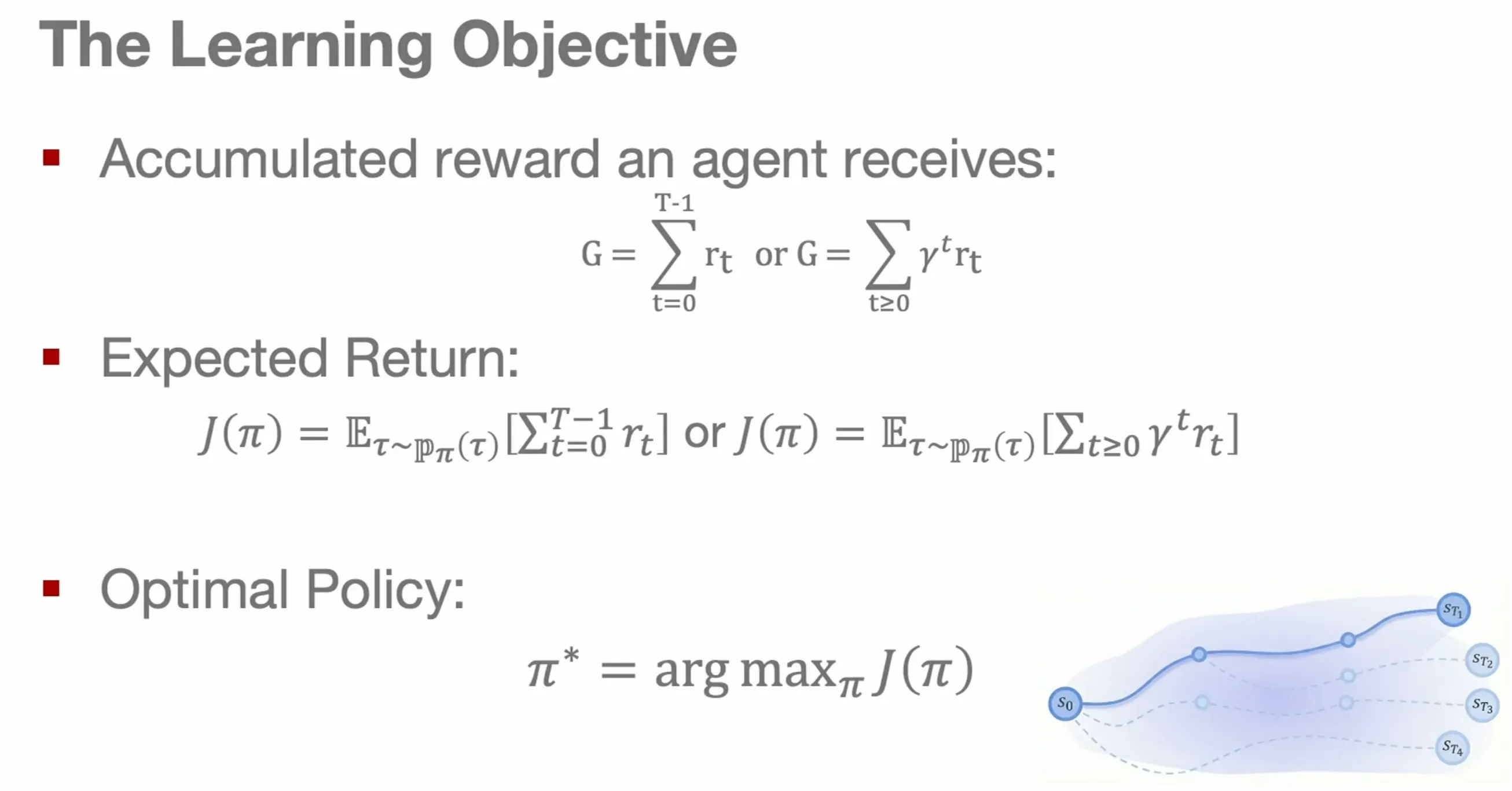
Finite-horizon vs infinite-horizon MDPs

• Finite-horizon MDPs: the episode ends after a fixed number of steps .
• Infinite-horizon MDPs: the episode can go on indefinitely, and we introduce a discount factor to ensure that the total reward is finite so the robot doesn’t just keep trying to maximize reward forever without ever stopping.

Learning objective

The optimal policy is the one that maximizes the expected return, which is the sum of discounted rewards over time. We can’t straight up use total reward because the world is stochastic, so we need to take the expectation over all possible trajectories that could occur under the policy.