CS 4432: Database Systems II

• Introduction

  • IO devices and latency --- PlanetScale

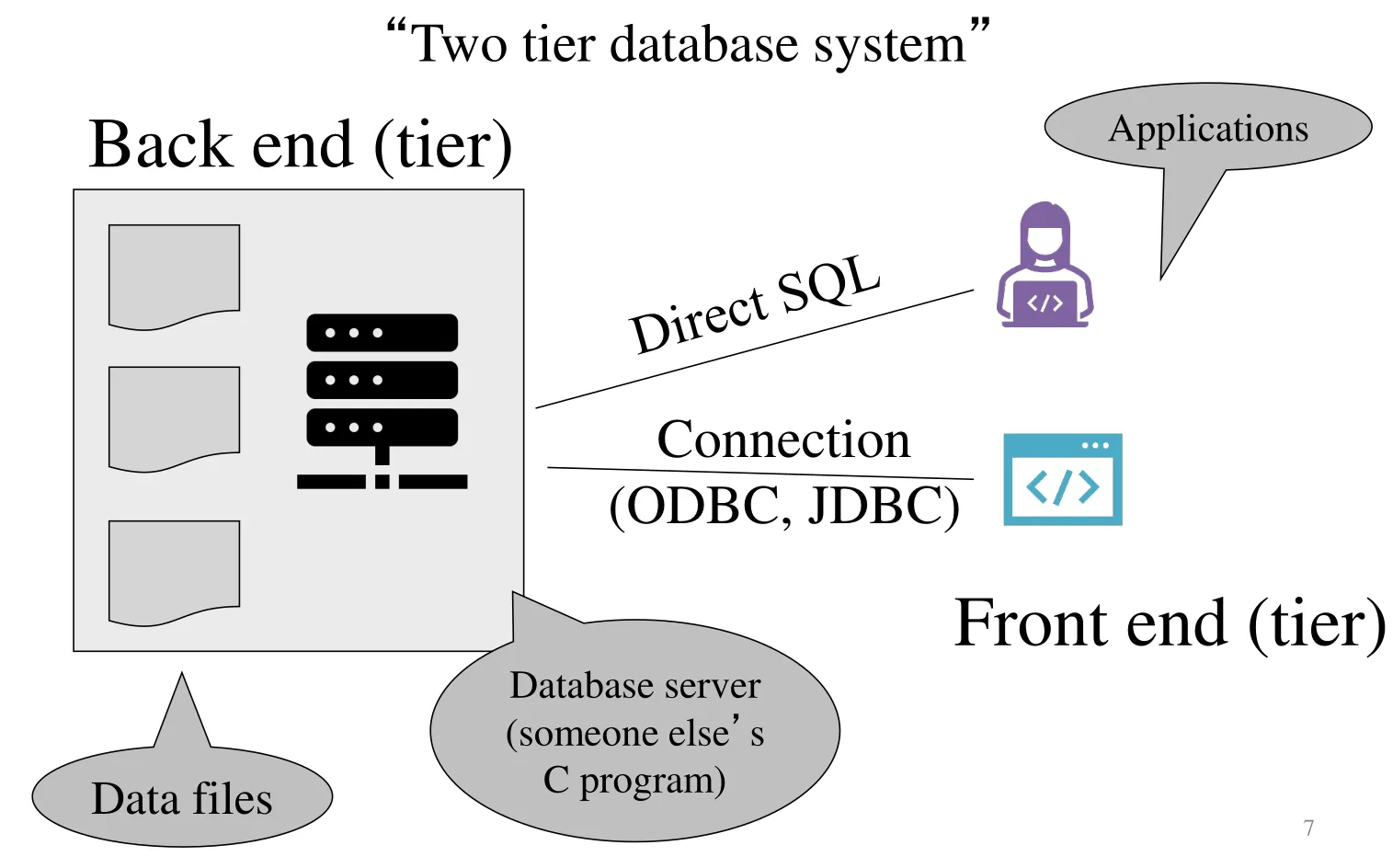
  • RDBMS

    • A collection of files that store the data

      • But: Files that we do not directly access or read

    • A big C program written by someone else that accesses and updates those files for you

      • But: Huge program containing 100s of 1000s of lines

• Structure

  • Frontend: SQL

    • Data Definition Language - DDL

    • Data Manipulation Language - DML

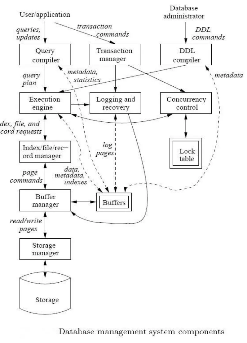
  • Backend

    • Query optimizer

    • Query engine

    • Storage management

    • Transaction management (concurrency, recovery)

• Abstraction

  • Tables (logical) → Creating file (data), may create indexes, updating catalog tables, read and update files on disk, check constraints (physical)

  • Queries (logical, declarative) → Imperative query execution plan

    • Complex cost model and many alternatives

    • The optimizer chooses the best execution plan for a query (may involve indexes)

  • Indexes (logical, declarative) → Create a index file, create a specialized data structure, whenever the data changes, the index has to be updated

  • Transactions (logical) → Concurrency control and logging and recovery control to ensure ACID properties

• File & System Structure: Records in blocks, dictionary, buffer management

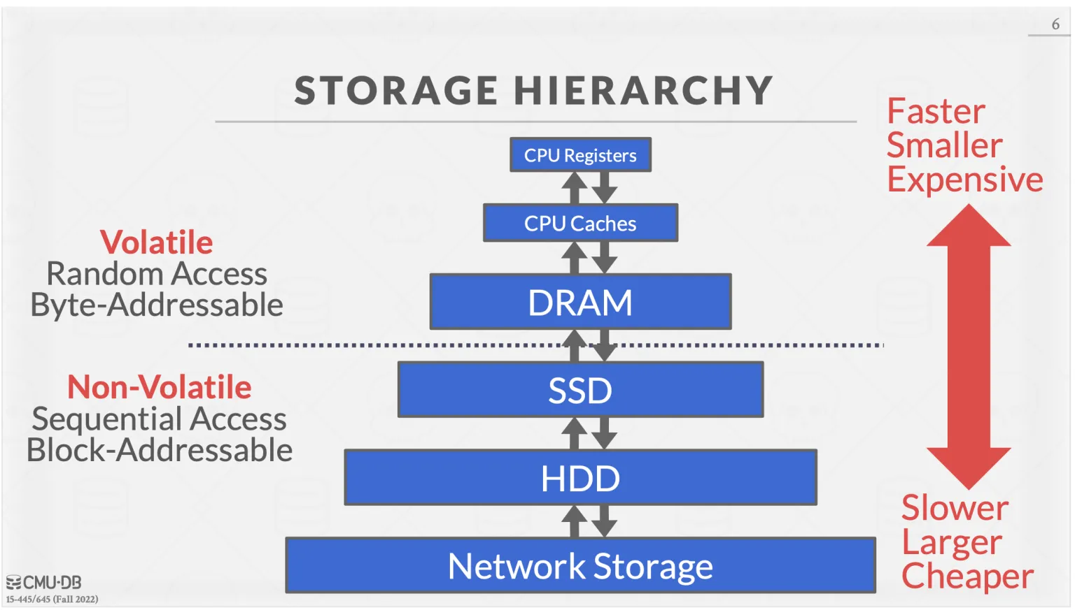
  • Disks and files

    • DBMS stores info on disks

    • Main memory is only for processing

    • Major implications on their design

      • READ: transfer data from disk → main memory

      • WRITE: transfer data from RAM → disk

      • High-cost operations (I/O) relative to in-memory operations

    • OS may take away memory in use by DBMS mid-operation (joining tables)

      • Why DBMS has storage manager and buffer manager

• Latency Numbers Every Programmer Should Know

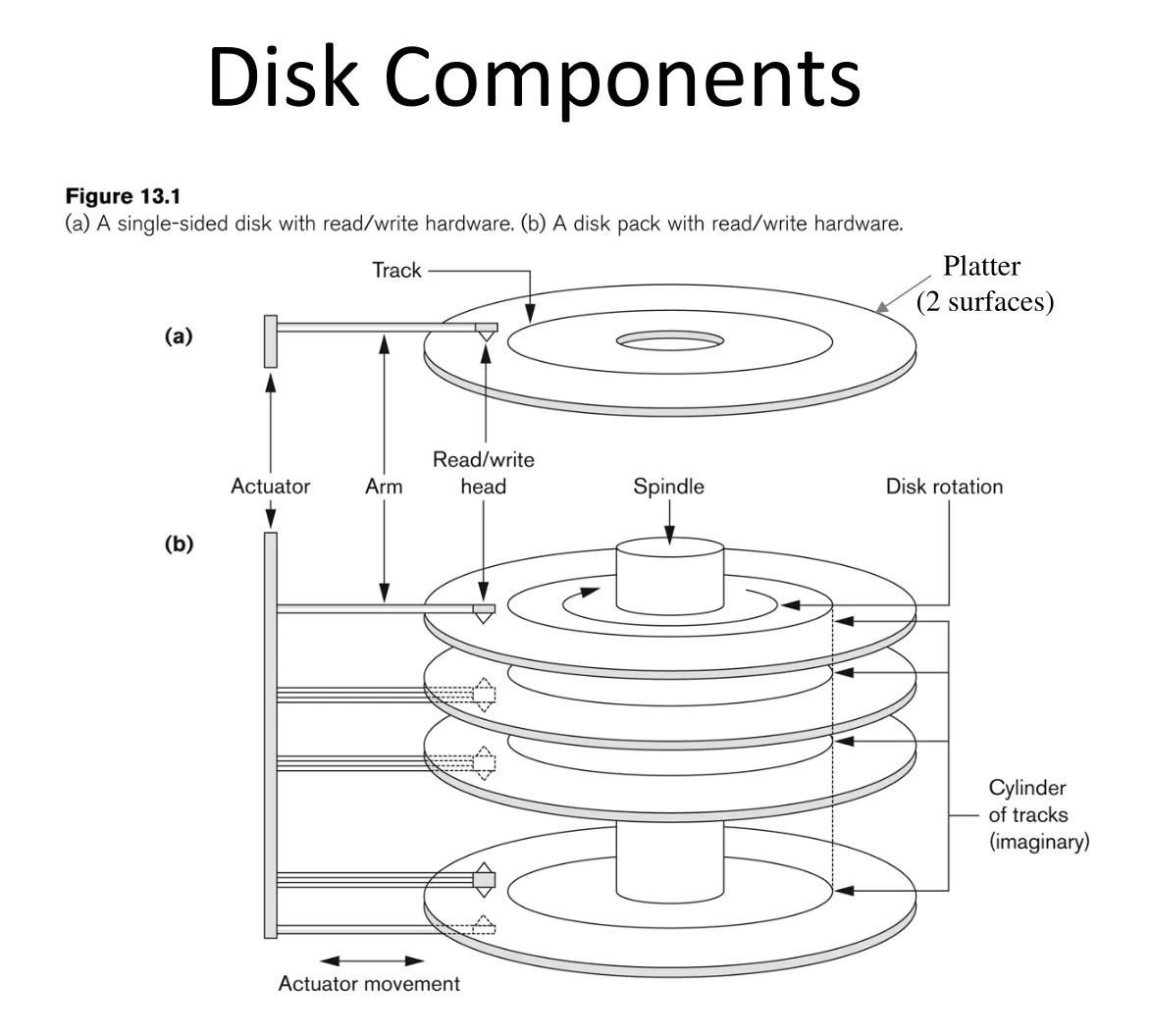
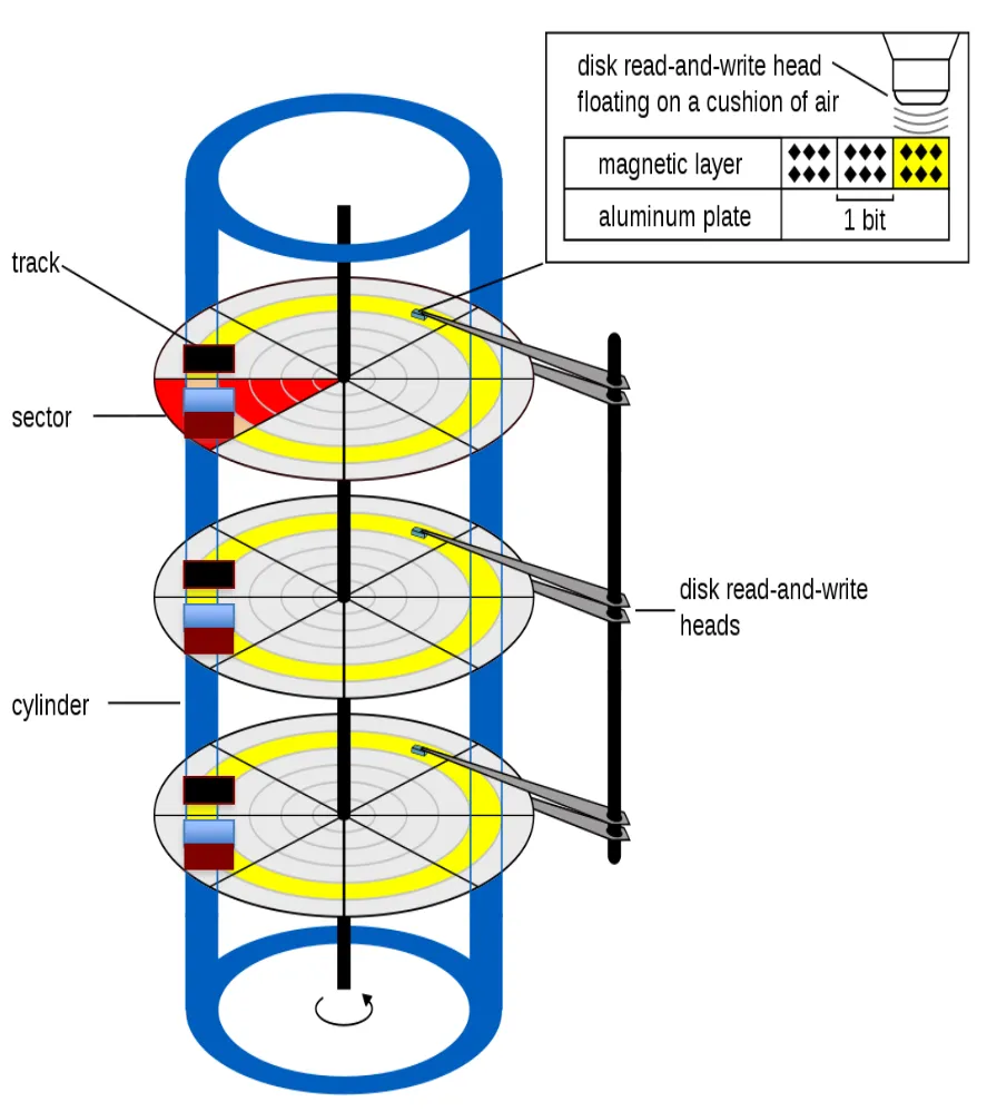
• Disks

  • Data is stored and retrieved in units called disk blocks (sometimes also referred to as “pages”)

  • Disk block typically between 4KB to 8KB

  • Movement to main memory

    • Must read or write one block at a time, meaning all R/W heads move together across tracks

    • Only one head is active at a time during a read/write operation

• Movements

  • Arm moves in-out

    • Called seek time

    • Mechanical

  • Platter rotates

    • Called latency (or rotation) time

    • Mechanical

• Sequential I/O typically costs less than random I/O because of less rotation time (all blocks sit next to each other on a track)

  • Read two random blocks

    • 2 seek times

    • 2 latency times

    • 2 transfer times

  • Read two blocks in a sequence

    • 1 seek time

    • 1 latency time

    • 2 transfer times

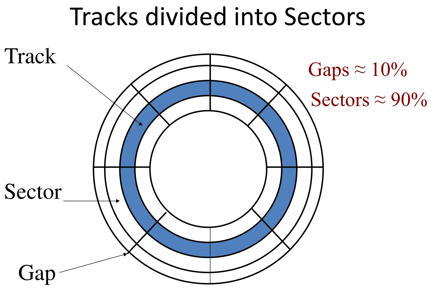
• Data storage

  • Size = 2 * num of platters * tracks * sectors * bytes per sector

    • 1KB = 1024 bytes

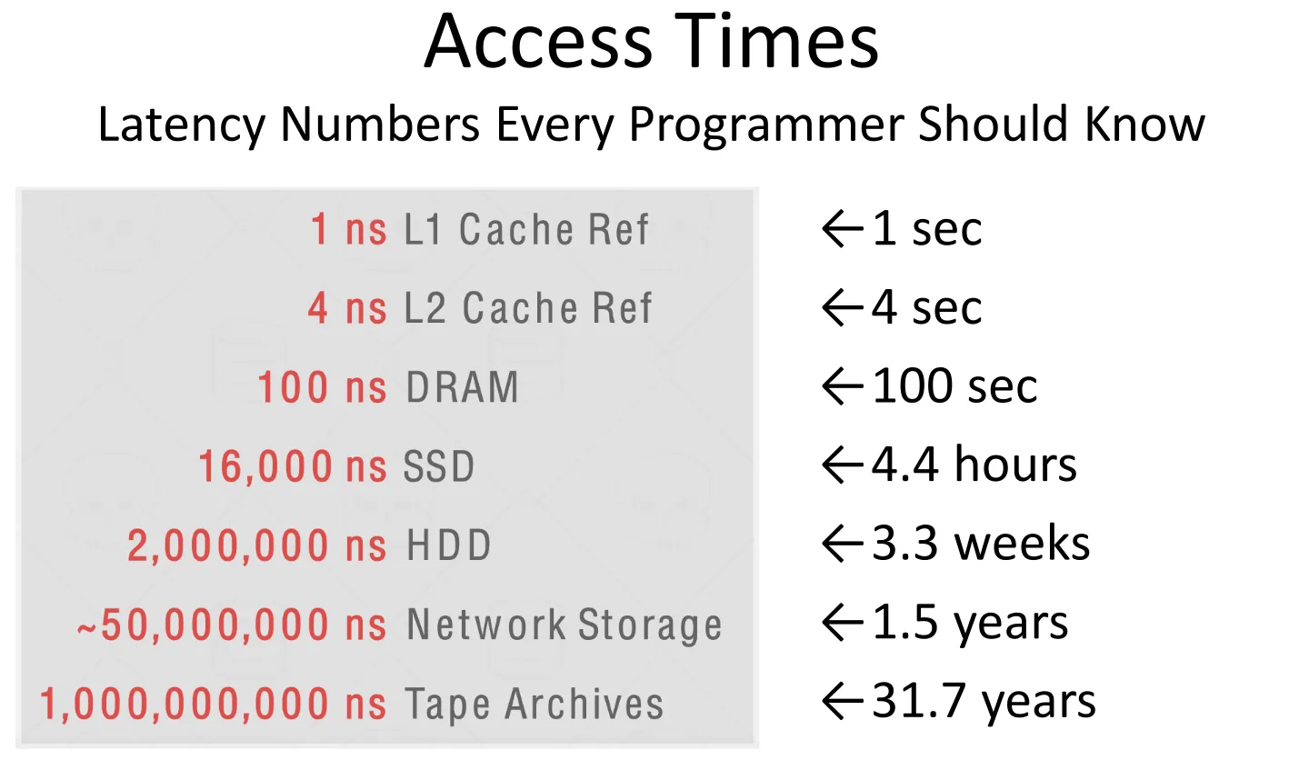
  • Accessing disk block latency = seek time (warm-up + travel) + latency (rotational) time + data transfer time

    • Average seek time = time to travel half of the number of tracks on a platter surface

      • ~9ms, ~4ms for high-performance drives

    • Average rotational latency = half of the time to make one full rotation

      • 10,000RPM = 3ms for newer drivers

    • Transfer time

      • 100-200MB/sec

      • Reading 4K data block takes ~0.02-0.04ms

      • Very small relative to seek and rotation time

    • Key to lower I/O cost: reduce seek/rotation latency → Sequential I/O

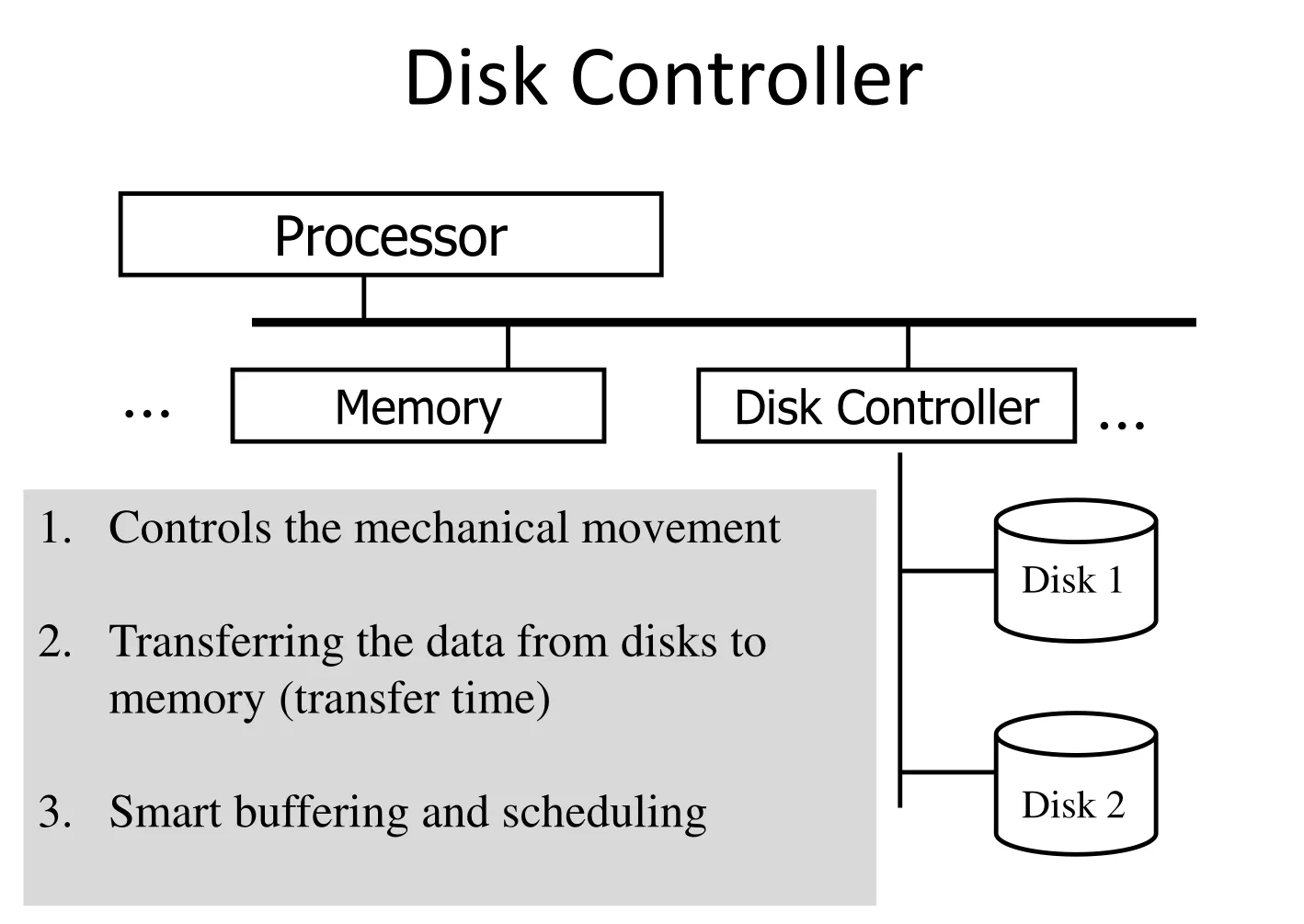
  • Accelerating access to blocks: performed by Disk Controller

    • Hardware component on the HDD that is responsible for managing data transfer

    • Main techniques

      • RAID: Redundant Array of Independent Disks: techniques used to improve storage performance, reliability, or both

        • Combines multiple physical disks into a single logical unit for redundancy and performance

        • Techniques: striping, mirroring, and parity

        • Several RAID levels

  ---

  RAIDDescription** Redundancy Performance Storage Use Case Level Efficiency**

  ---

  RAID 0 Striping None High 100% Non-critical, high-speed tasks

  RAID 1 Mirroring High Moderate 50% Critical data, system drives

  RAID 5 Striping with Medium Good (N-1)/N General-purpose Parity storage

  RAID 6 Striping with High Moderate (N-2)/N High-reliability Double Parity storage

  RAID 10 Mirroring + High High 50% High-performance, Striping critical data

  ---

• Placing related blocks on same cylinder

  • Put on the same cylinder to read them at once

  • Make use of the 2 surfaces in the same cylinder

  • Add more blocks on the next sectors on the same track

  • “At once” meaning “one at a time but really fast” because transfer time <<< rotation time

• Using multiple disks: Striping (RAID 0)

  • Use multiple smaller disks instead of one larger disk

  • Each disk can access data independently, in parallel

    • N disks → N times faster access

• Mirroring (RAID 1)

  • Use pair of disks that mirror each other

  • Good for durability but higher overhead for writing

• Disk scheduling

  • Disk Controller holds a sequence of block requests (queue of requests)

  • Not necessarily serve requests in their arrival order (FIFO) ➔ Use better scheduling policy

  • Elevator (SCAN) policy

    • Purpose: Optimize disk read/write head movement.

    • Mechanism:

      • Moves in one direction (e.g., inward to outward or vice versa).

      • Services all requests along the path in the current direction.

      • Reverses direction at the end of the disk.

    • Advantages:

      • Fairness: Services requests at both ends of the disk.

      • Reduces starvation compared to FCFS.

    • Disadvantages:

      • Overhead: May travel to the end unnecessarily.

      • Latency: Requests at the far end may wait longer.

    • Example:

      • Cylinders: 0 (inner) to 199 (outer).

      • Head at 50, moving outward.

      • Requests: [10, 60, 80, 120, 30].

      • Services: 60 → 80 → 120 → (reverses) → 30 → 10.

    • Efficient and fair, but may incur overhead due to unnecessary disk arm movement

• Prefetching and buffering

  • If DBMS can predict the sequence of access, it can pre-fetch and buffer more blocks even before requesting them.

  • Naive single buffer algorithm

    • Say a file has sequence of blocks B1, B2,… and a program that process B1, B2, B3,…

    • Execution of algorithm

      • (1) Read B1 → Buffer

      • (2) Process Data in Buffer

      • (3) Read B2 → Buffer

      • (4) Process Data in Buffer

    • Cost: n(P+R)

      • P: time to process a in-memory block

      • R: time to read disk block (seek + latency + transfer)

      • n: # of blocks

  • Double buffering

    • Purpose: Overlap I/O operations with computation to reduce idle time.

    • How it works:

      • Two in-memory buffers are used: Buffer A and Buffer B.

      • While the CPU processes data in Buffer A, the I/O system loads data into Buffer B.

      • Once the CPU finishes processing Buffer A, it switches to Buffer B, and the I/O system loads new data into Buffer A.

    • Advantages:

      • Reduces CPU idle time by overlapping I/O and computation.

      • Smooths out performance for real-time systems (e.g., video playback).

  • Prefetching

    • Purpose: Reduce latency by loading data into memory before it is needed.

    • How it works:

      • The system predicts which data will be needed next and loads it into memory in advance.

      • Prefetched data is stored in a buffer or cache.

    • Advantages:

      • Hides memory or disk latency by overlapping data transfer with computation.

      • Improves performance for sequential or predictable access patterns.

  • Combining double buffering and prefetching

    • While the CPU processes data in Buffer A, prefetching loads data into Buffer B.

    • When the CPU switches to Buffer B, prefetching loads the next set of data into Buffer A.

  • Cost: R + nP

    • Have to pay R for the first block

    • Assuming sequential I/O, time to read other blocks is very small compared to P

    • Time to retrieve them overlaps with nP

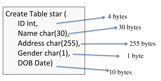
• Record representation

  • Database records (tuples)

    • Each record, and each field is just a sequence of bytes on a disk block

    • Field has type that can be fixed- or variable- length

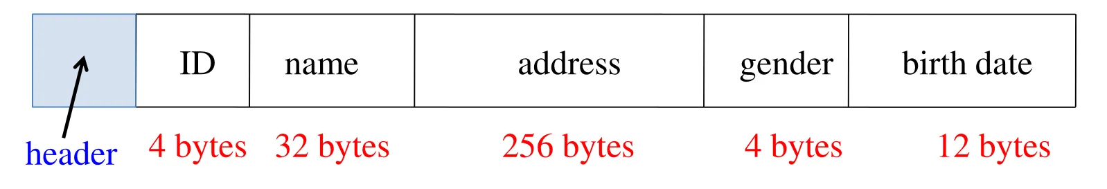
    • All fields in a record are aligned to start at 4- or 8-byte boundaries & concatenated

• Each record has a header holding some info

• Two types of records: fixed-length and variable-length

  • Different fixed-length records have the same size

  • Different variable-length records may have different sizes

    • VARCHAR (variable characters), VARBINARY, TEXT, BLOB, JSON/XML

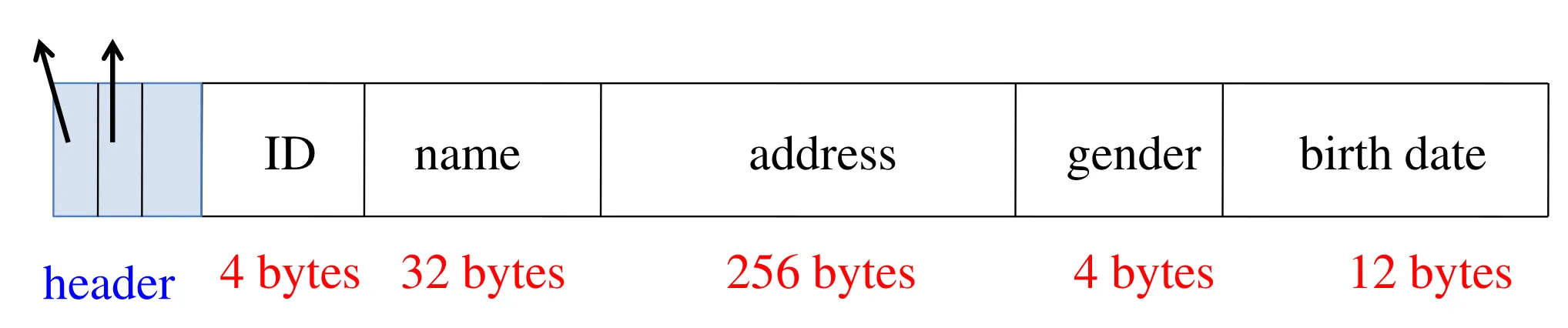
• Record header

  • Often it is convenient to keep some “header”

  • information in each record:

    • A pointer to schema information (attributes/fields, types, their order in the tuple, constraints)

    • Length of the record/tuple

    • Timestamp of last modification

• Packing records into blocks

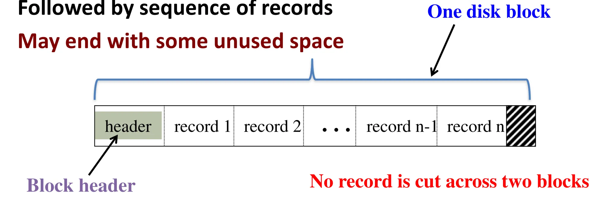
  • Start with a block header

  • Followed by sequence of records

  • May end with some unused space

  • No record is split between blocks

• Accessing fixed-length records

  • Information about field types are the same for all records in a file; stored in system catalogs

  • Finding i’th record in a block does not require scan over previous records

  • Finding i’th field does not require scan over previous fields

• Records with variable-length fields

  • A field whose length can be different across records

  • Complicated design and access, but sometimes efficient to have

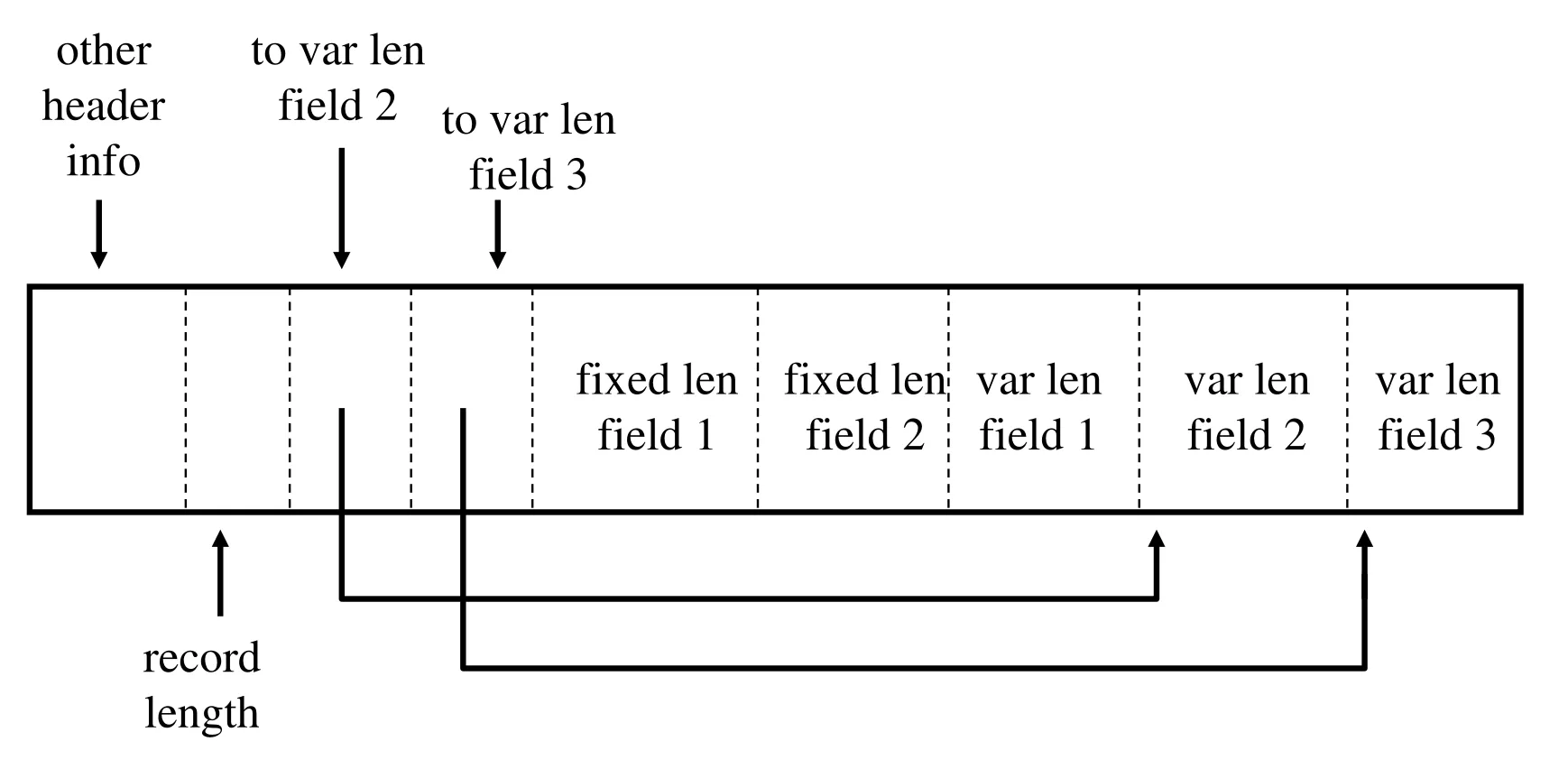
  • Effective representation

    • Fixed length fields are kept ahead of the variable length fields

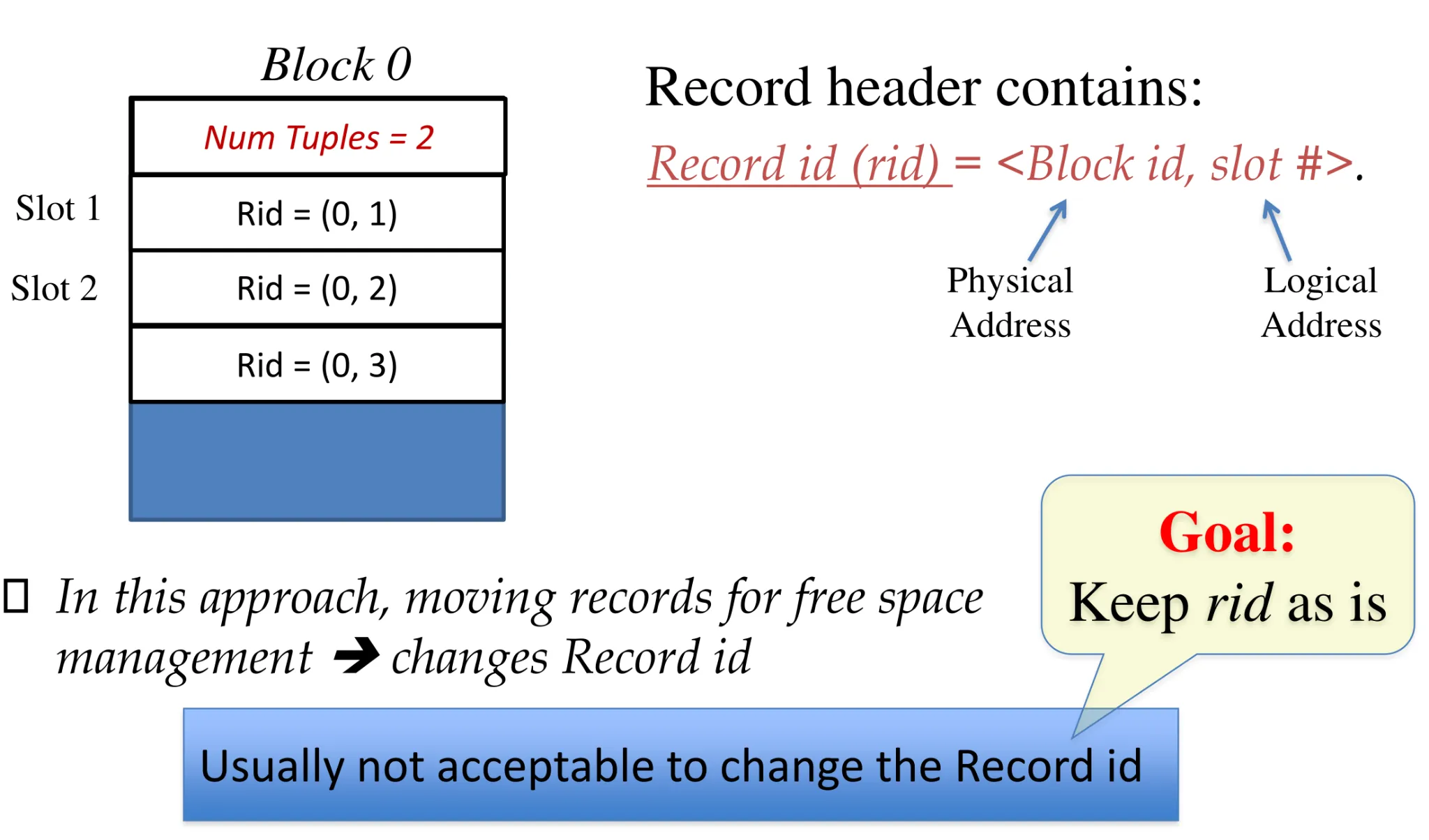
    • Record header contains

      • Record length

      • Pointers to beginning of each variable length field except the first one

• Efficient access → still reading i’th record without scanning over previous fields

• Packing records into blocks

  • Packed approach (fixed-length records)

    • Packed means no holes between records

    • Insertion

      • If enough free space at the end the insert in this block

      • Increment number of tuples in block header

    • Deletion

      • Move the last record to fill in the empty space

      • Decrement N

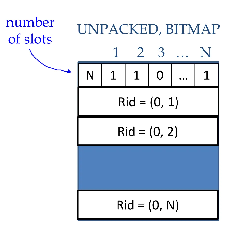
• Bitmap/unpacked approach (fixed-length records)

• Insertion

  • Find free slot anywhere in the block

  • Insert the record

  • Increment N

  • Set its free bit to 1

• Decrement

  • No copying/movement

  • Decrement N

  • Set its bit to 0

• Better approach, but does not work for variable-length records

• Variable-length records

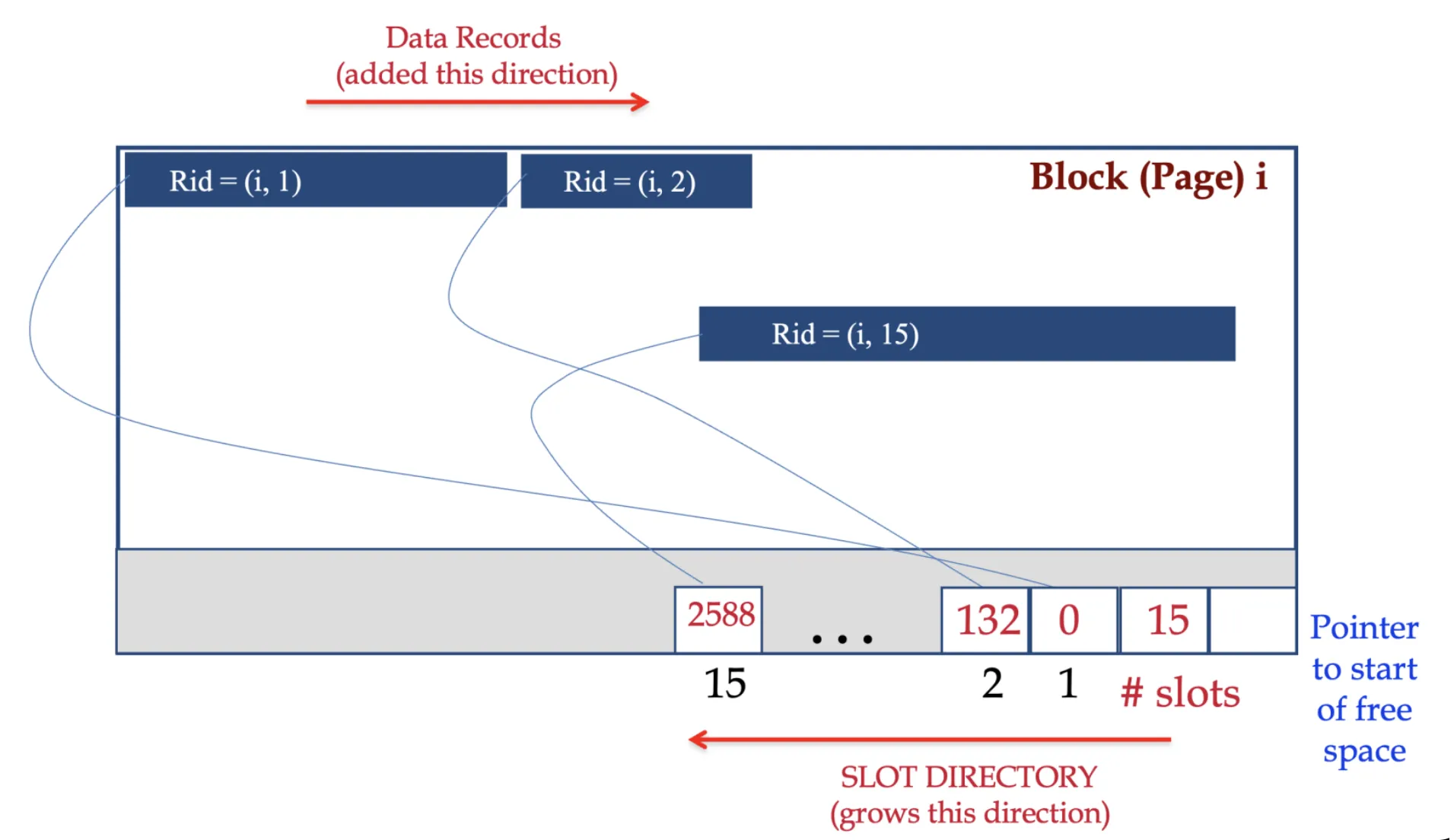
• The slot directory starts from one end and grows as needed

• The data records start from the other end (No need for fixed allocation for SLOT directory)

• Rid does not change even if the record moves within the block

• Deleting a record will leave some empty space in the middle

• Buffer manager

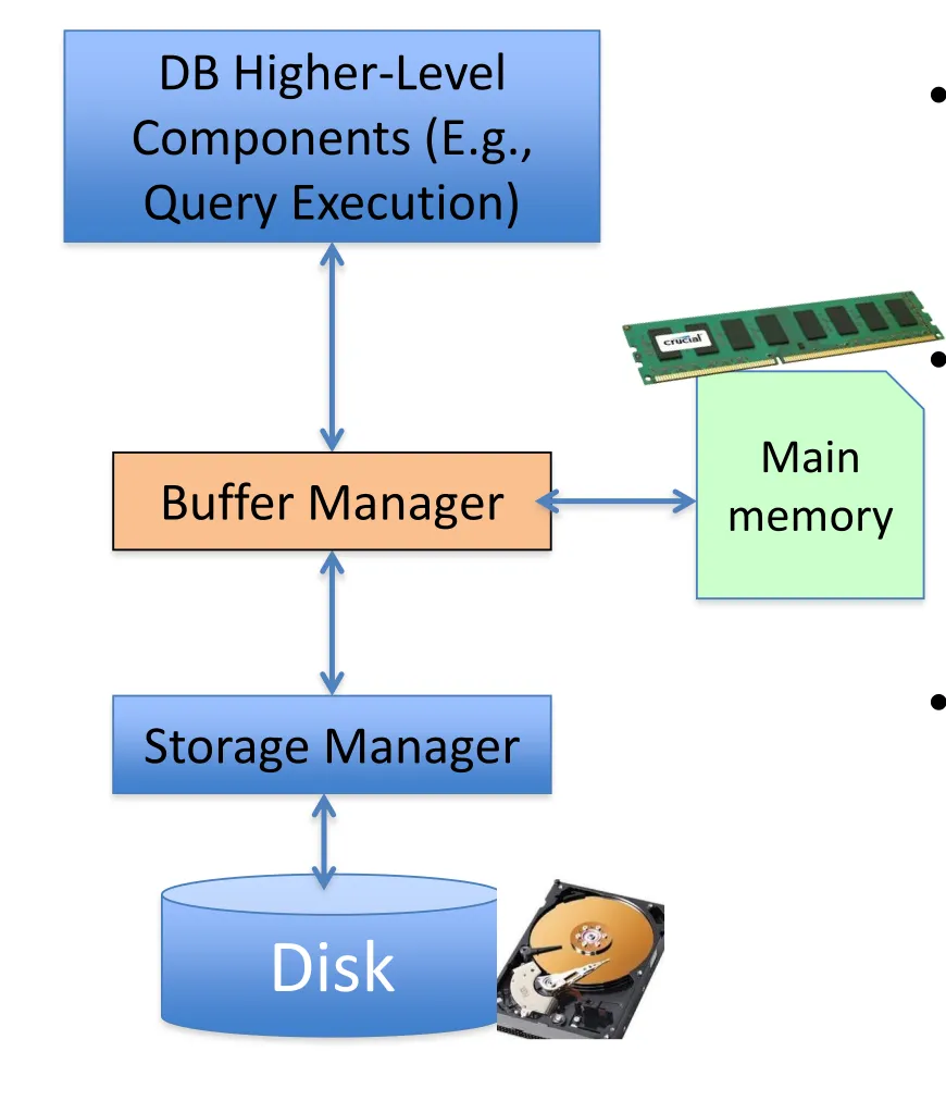
• Index/file/record manager issues page commands to buffer manager

• Buffer manager manages what blocks should be in memory and for how long

  • Computations/modifications on/to data pages can only be made when they are in main memory, NOT on disk

• Insight: [https://chatgpt.com/share/67e6ed51-0ea0-800b-8680-f5e888d3780b]](https://chatgpt.com/share/67e6ed51-0ea0-800b-8680-f5e888d3780b)

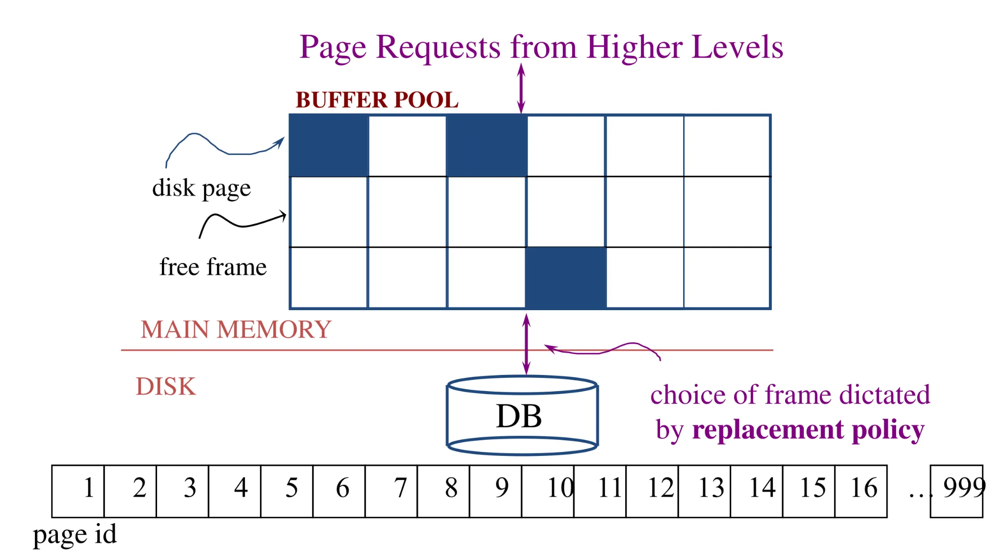
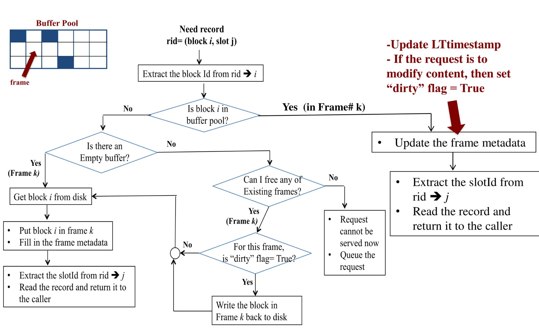
• Buffer pool

  • Array called buffer pool, each entry is called frame

  • Buffer pool information table contains: <frame number, disk page ID, pin count, dirty>

    • Dirty: whether the content has changed

    • Pin: can be taken out if need and count = 0, else has to stay in-memory until unpinned

    • LTTimestamp: last touched (R+W) timestamp

  • Each entry can hold 1 database disk block

    • An in-memory disk block is a.k.a. memory page

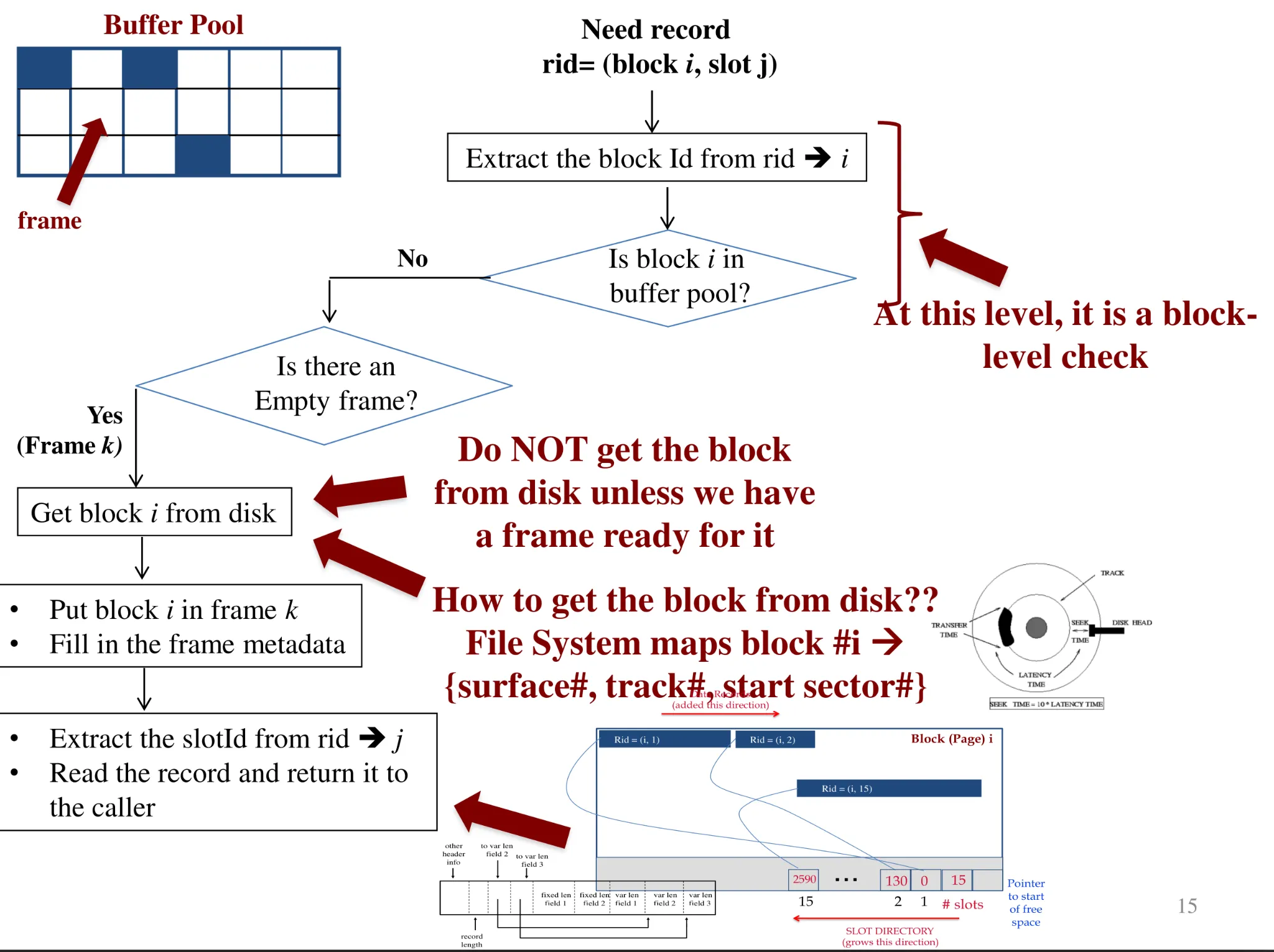
  • Buffer manager keeps track of

    • Which pages are empty

      • Naive: scan array of frames looking for blockId -1 (O(n))

      • Better: array of empty frames

      • Even better: bitmap of which frames are used (O(1))

    • Which disk page exists in which frame

      • Naive: scan array of frames looking for blockId i (O(n))

      • Better: hashmap blockId → frame number (O(1))

        • No need to keep blockId in frame metadata anymore

• How do we choose which frame to free among the unpinned ones? Buffer replacement policies

  • LRU, FIFO, clock replacement algorithm

  • Have a big impact on number of I/O’s → depending on the access pattern

  • Also may need additional metadata to be stored for each frame

  • LRU

    • For each frame in buffer pool, keep track of time when last accessed ➔ (LTtimestamp)

    • Replace the frame which has the oldest (earliest) time

    • Very common policy: intuitive and simple

      • Works well for repeated accesses to popular pages

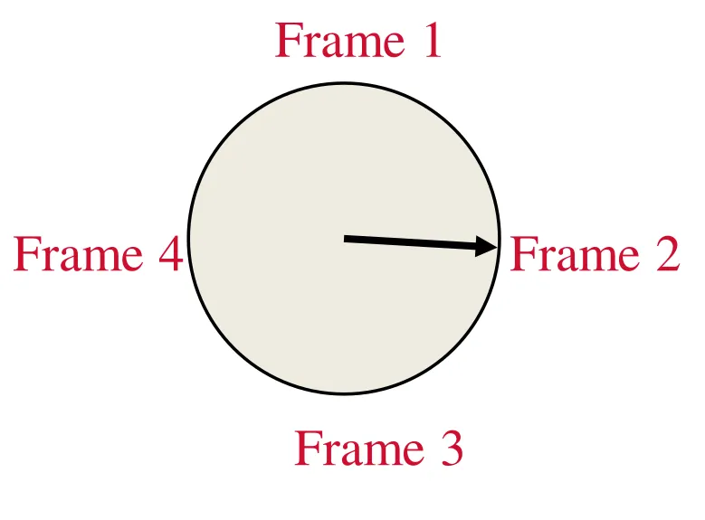
  • Clock

    • An approximation of LRU

    • Each frame has

      • Pin count ➔ If larger than 0, do not touch it

      • Ref bit (second chance bit) ➔ 0 or 1

    • Imagine frames organized into a cycle

    • A pointer rotates to find a candidate frame to free

      • IF pin-count > 0 Then ➔ Skip

      • IF (pin-count = 0) & (Ref = 1) ➔ Set (Ref = 0) and skip (second chance)

      • IF (pin-count = 0) & (Ref = 0) ➔ free and re-use

    • Need additional metadata

      • Second chance (reference bit)

    • Small overhead

  • Problem: sequential flooding

    • Queries can involve repeated sequential scans

    • # free buffer frames < # pages in file means some page requests cause an I/O.

    • High cost ➔ Each access modifies the metadata

    • Affects both LRU and Clock Replacement

• Pinning memory pages

  • Pinning a page means not to take from the memory until unpinned

  • Why pin a page?

    • Keep it until the transaction completes

    • Page is reference a lot

    • Recovery control

    • Concurrency control (enforcing certain order)

  • Releasing unmodified pages

    • When done with a page

      • Unpin the page (if you can)

      • Since page is not modified → claim this page in the free list

      • No need to write back to disk

  • Releasing modified pages: have to notify the disk manager to modify the corresponding on-disk block afterward

• Sorting in main memory

  • In DBMS, the data can be much larger than main memory

  • Why sort?

    • Data requested in sorted order

    • Many DB operations require sorting

  • Using secondary storage effectively

    • General wisdom

      • I/O costs dominate

      • Design algorithms to reduce I/O

      • CPU overhead becomes less important

  • Merge sort

    • In-memory: EZ

    • Externally (using disk)

      • How many memory buffers are needed?

      • What is the I/O cost?

      • 2-way external sort (Naive method)

      • Phase 1: Prepare

        • Read a page, sort it, write it

        • Only one buffer page is used

      • Phase 2, 3…(recursively): Merge two sub-lists in each phase

        • Three buffer pages used

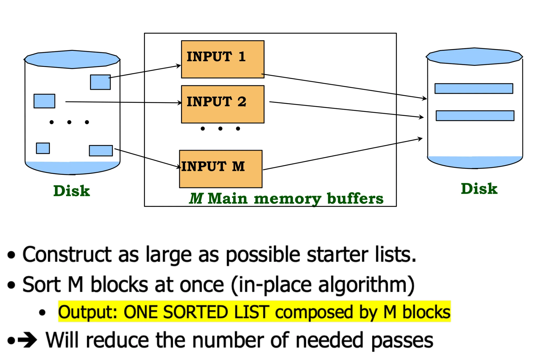
• M-way external sort

  • Sorting a file with N pages using M buffer pages

  • Pass 0: use M buffer pages.

    • Produce N/M sorted runs of M pages each.

  • Pass 1, 2, …, etc.: merge M-1 runs.

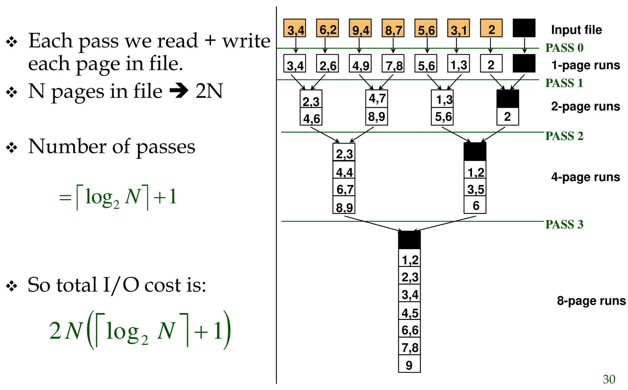
• Number of passes

• Total I/O cost = 2N * (# of passes)

• Summary

  • Use as much memory buffers you can

  • Cost metric

    • I/O only (till now)

    • CPU is nontrivial, worth reducing

      • Use a quick main-memory algorithm

  • For the in-memory sorting part

    • Use Quicksort or heapsort

• Indexing

  • Heap file of a relation: storage structure used to store the tuples (rows) of that relation without any specific order

  • Table scan: Naive way

    • Open the heap file of relation R

    • Access each data page

    • Access each record in the data page

    • Check the condition

    • I/O cost: O(N)

    • Memory needed: only 1 memory block

    • Index scans are more efficient, but requires DBMS to index the table beforehand

  • Concepts

    • Indexing is used to speed up access to desired data

    • Search key — attribute to set of attributes used to look up records in a relation (WHERE clause in the SQL query)

      • Example:

SELECT id, name, address

FROM R

WHERE id=1000; → Search key

• Index file

  • Consists of records (called index entries) of the format

• Typically much smaller than the data file it’s indexing

• Types of indexes

  • Dense vs sparse

  • Primary vs secondary

  • One-level vs multi-level

• Index evaluation metrics

  • Saves query times, but adds overhead to insertion, update/deletion, and space

  • Supported access patterns

    • Equality search (x = 100): records with a specified value in the attribute

    • Range search (10 < x < 100): records with an attribute value falling in a specified range of values.

• Primary index

  • An index on the ordering column (the column on which the data file is sorted)

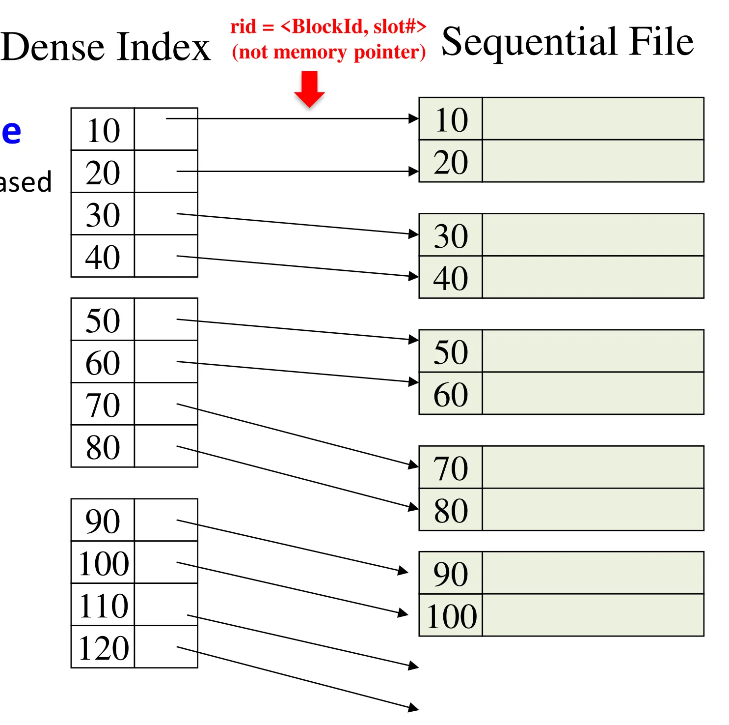
  • Dense index in ordered file

    • Ordered (sequential) files

      • Records are stored sorted based on the indexed attribute

    • Dense index

      • Has one entry for each data tuple

• Number of entries in index = records in file

• But index size is much smaller (since only 2 columns)

• Index scan

  • Read each page from the index

  • — Search for key = 100

  • — Follow the pointer ➔ (Record Id)

• Index binary search

  • Since all keys are sorted

  • Read middle page in index

  • Either you find the key, or

    • Move up or down

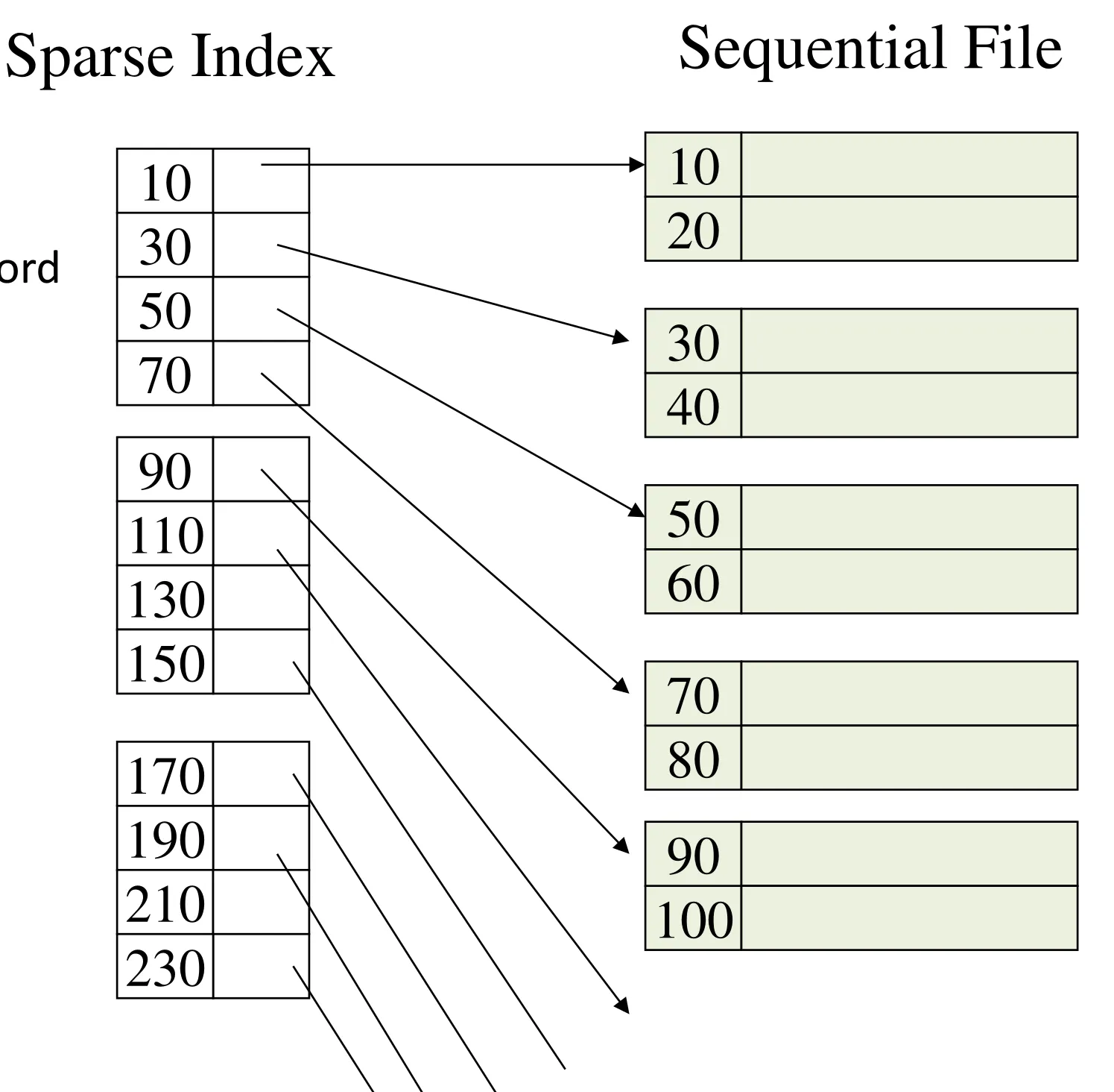
• Sparse index in ordered file

• Sparse index

  • An entry for only the 1rst record in each data block

  • Much smaller than a dense index

  • Can only be built on ordered (sequential) files

• Index binary search still works

  • Either locate the search key in the index, OR

  • Locate the largest key smaller than your search key

  • Follow the pointer and check the data block

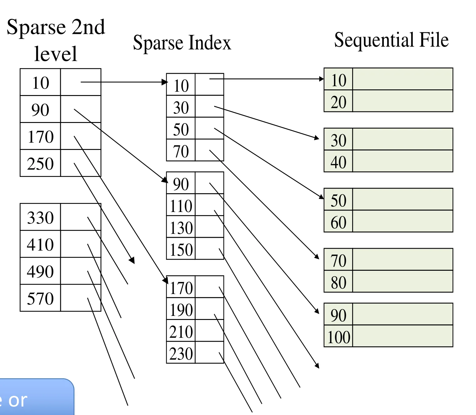
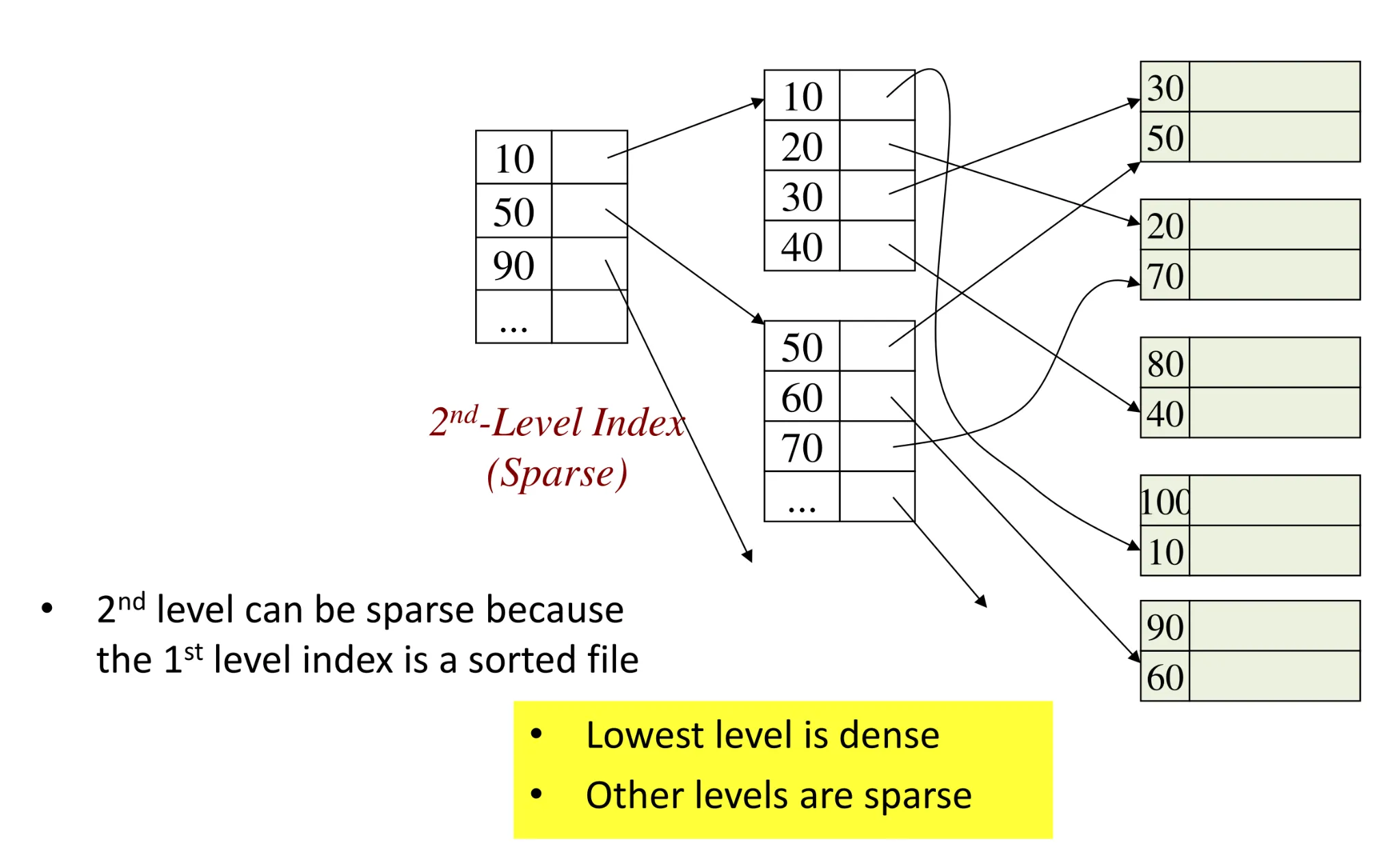
• Multi-level index

• 1st level Index file is just a file with sorted keys

  • We can build a 2nd level index on top of it

• Beyond the 1st level (which can be dense or sparse), all following levels should be sparse to save on space

• Sparse vs dense index

  • Sparse

    • Less space

    • Only for sorted files or higher-level indexes

    • Better for insertion

    • Cannot tell if record does not exist without checking data file

  • Dense

    • More space

    • Must use for unsorted files (secondary indexes)

    • Can tell if record does not exist without checking the data file

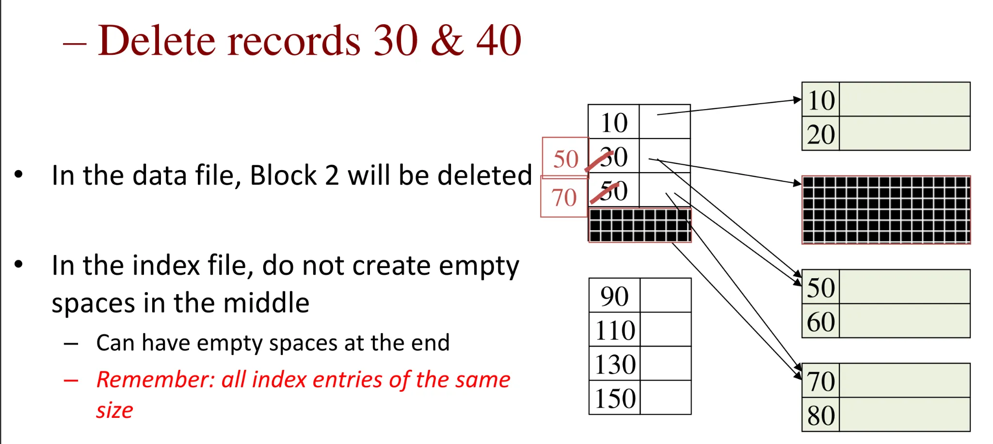
• Insertion/deletion in ordered file

  • Sparse index: deletion

    • If deletion were not an indexed record, index requires no re-organization

      • Data blocks will have some empty space

    • If deletion were an indexed record (1rst entry in the data block), the search key value in the index entry will change to the new 1rst entry in the data block

      • The 1rst entry may or may not move

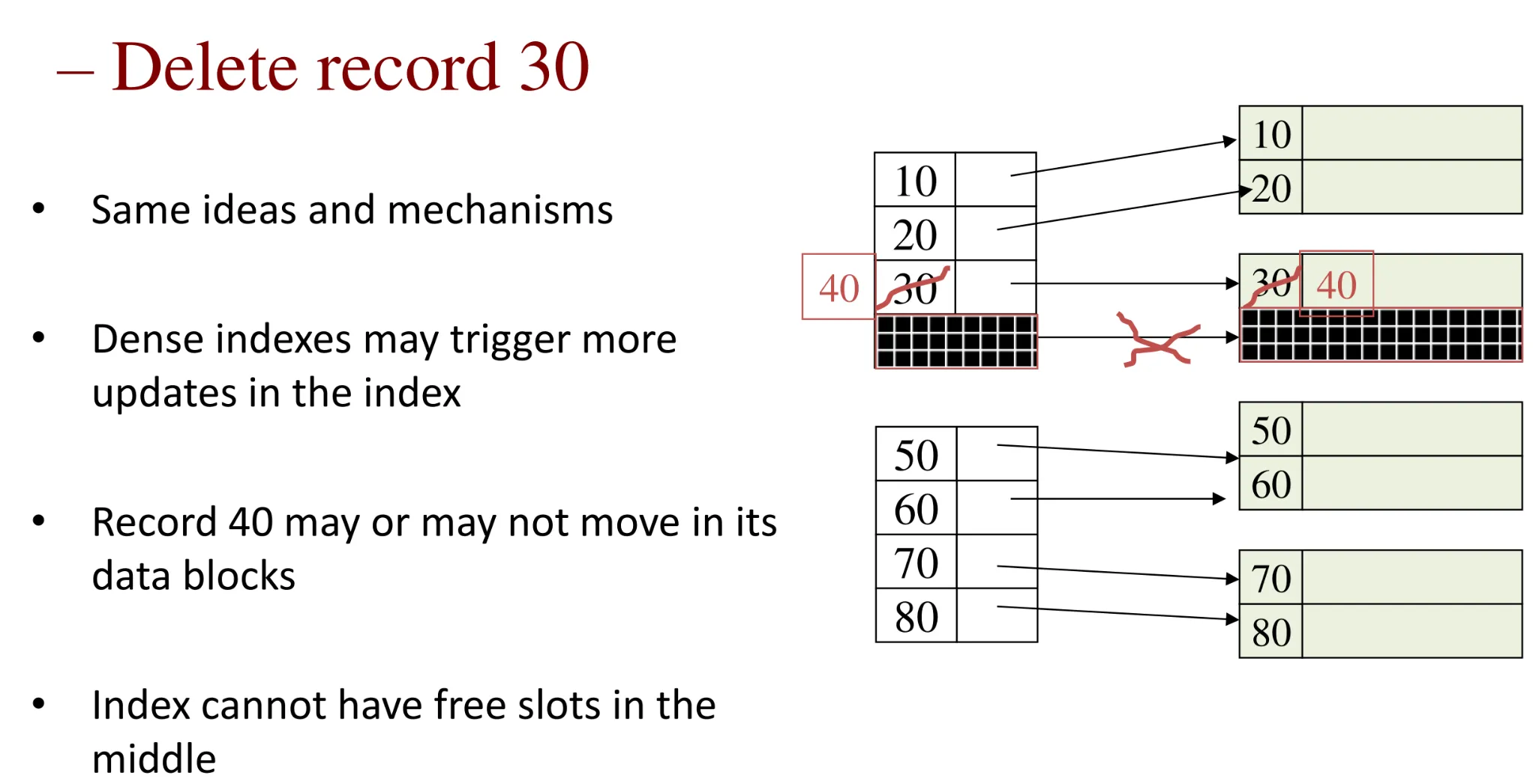
• Dense index

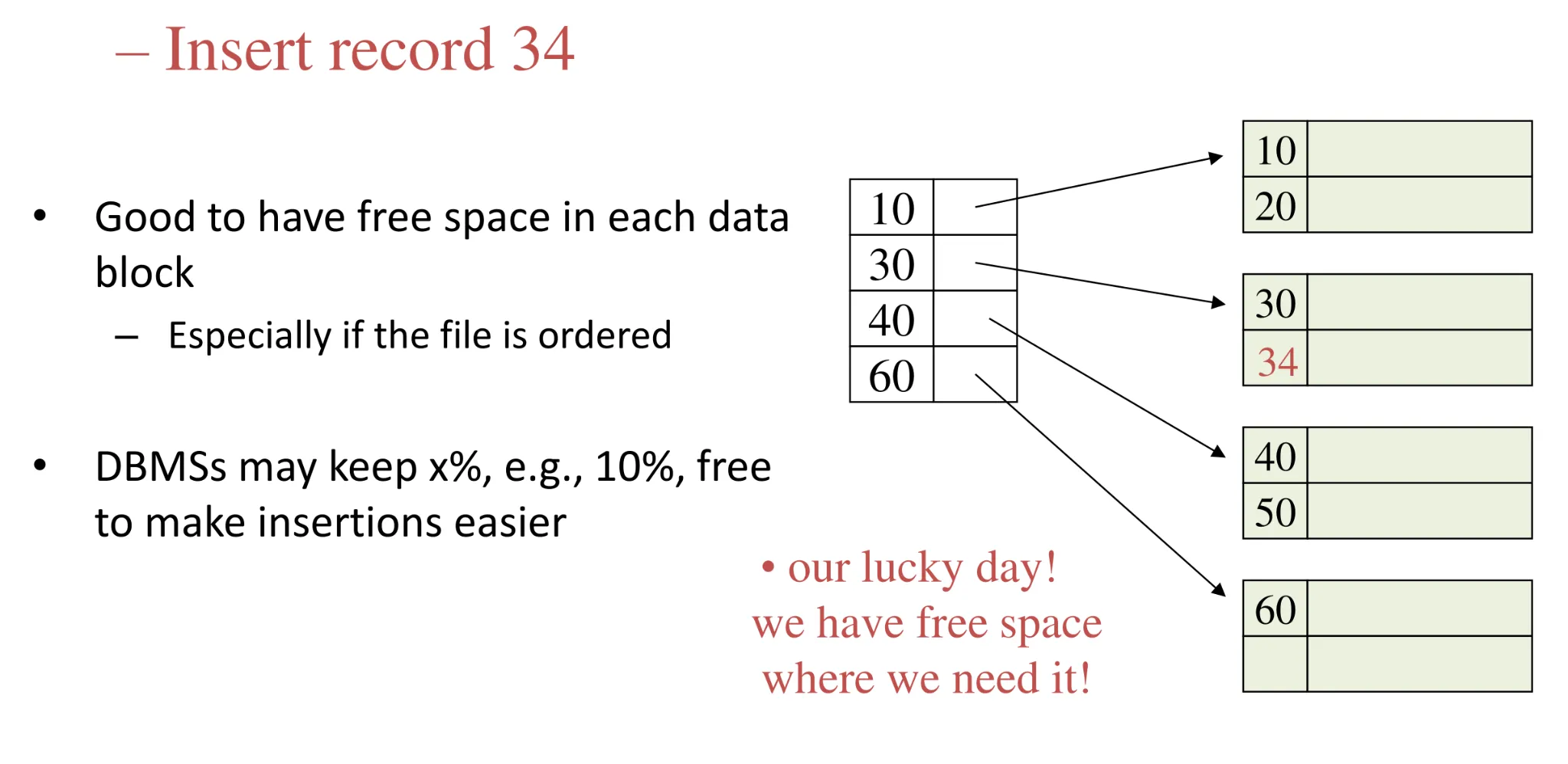
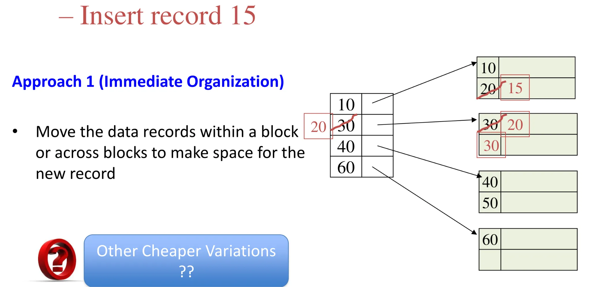
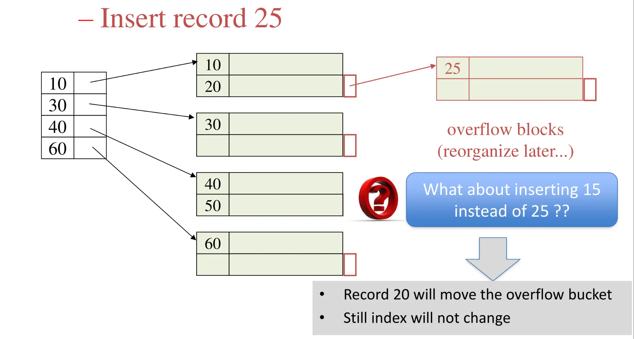
• Sparse index: insertion

• Use of overflow blocks

  • Overflow blocks are invisible to the index (do not affect the index entries)

• Dense index: insertion — similar, often more expensive

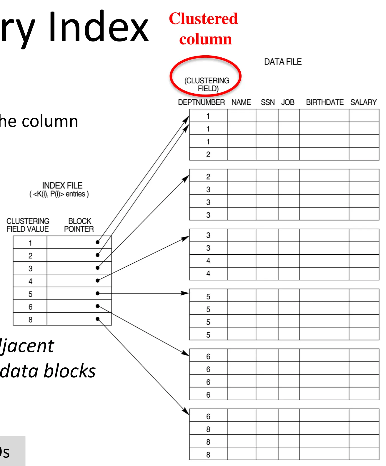
• Primary vs secondary index

  • Primary index

    • An index on the ordering column (the column on which the data file is sorted)

    • Can be dense or sparse

    • Can be one-level or multi-level

    • Big advantage

      • Records having the same key (or adjacent keys) are in the same (or adjacent) data blocks → Leads to sequential I/Os

• Unordered files

  • File where records are not ordered on the indexed column

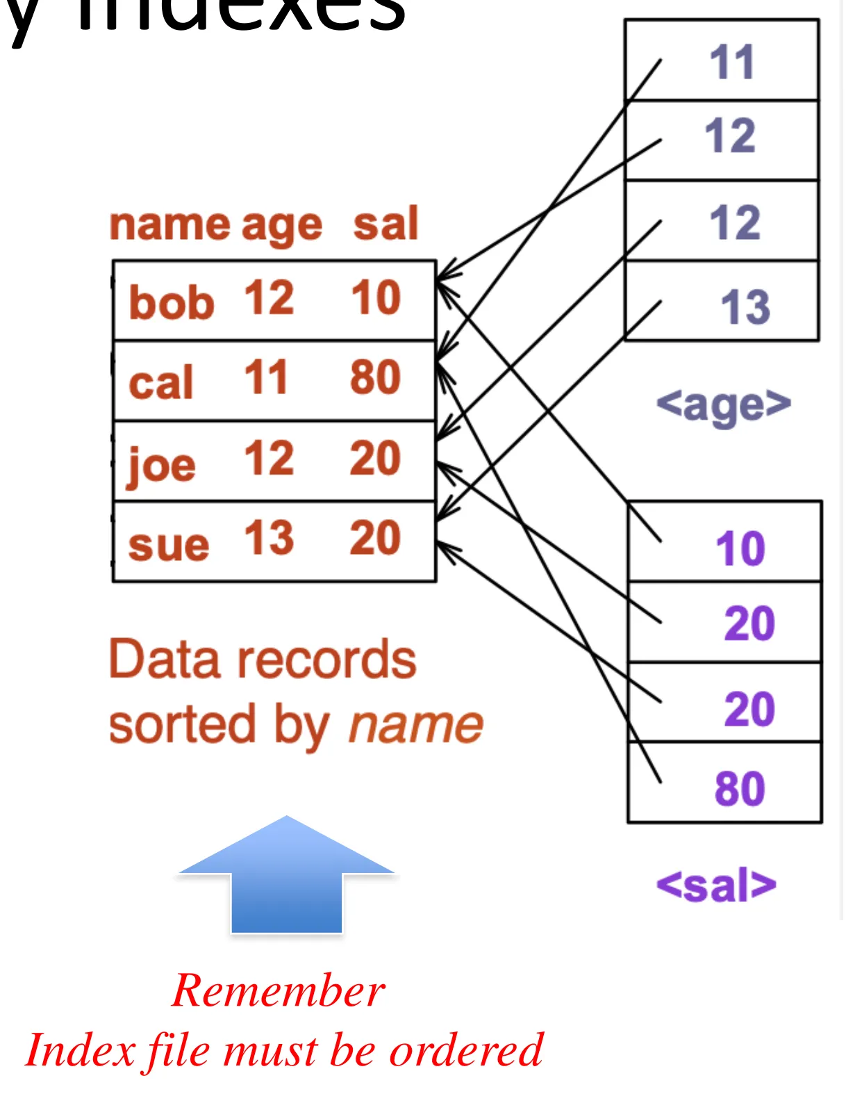
• Secondary index

  • An index on a relation’s unordered (physically) column

  • The file may be ordered on another column, say Name.

    • An index on the Name column is primary index (Can be sparse or dense)

    • An index on any other column, say ID, is called secondary index (can only be dense)

  • An index entry for each data record

  • Pointers will cause random I/Os (even for same or adjacent values)

• Multi-level secondary index

• Duplicate values

  • Option 1: typical dense index

    • Repeated keys can be many

    • Problem: excess overhead

      • Disk space

      • Search time

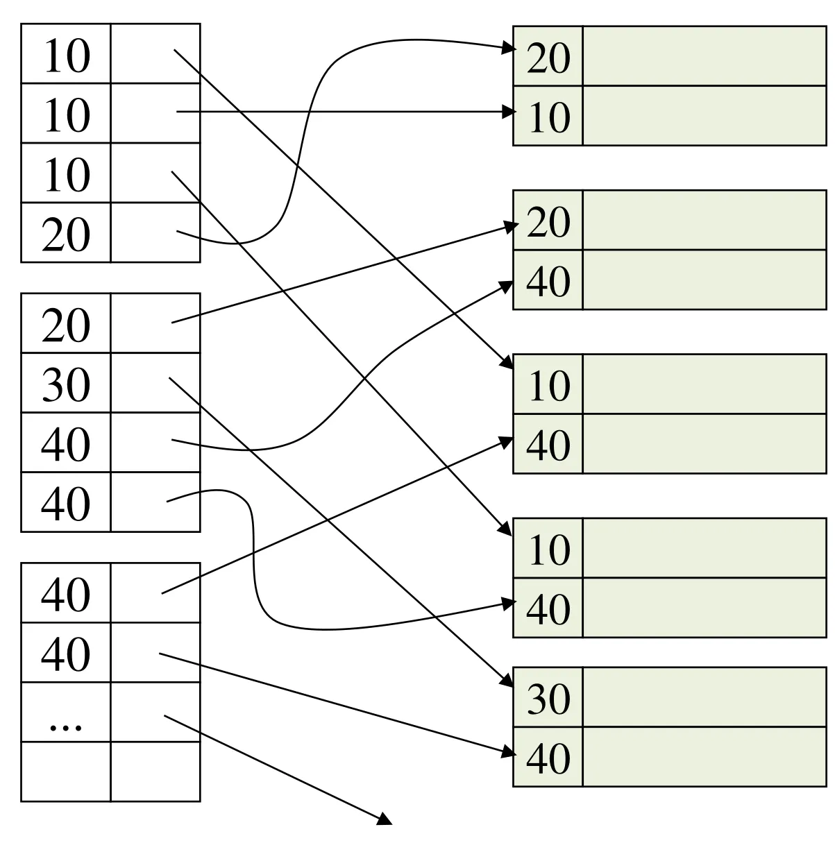
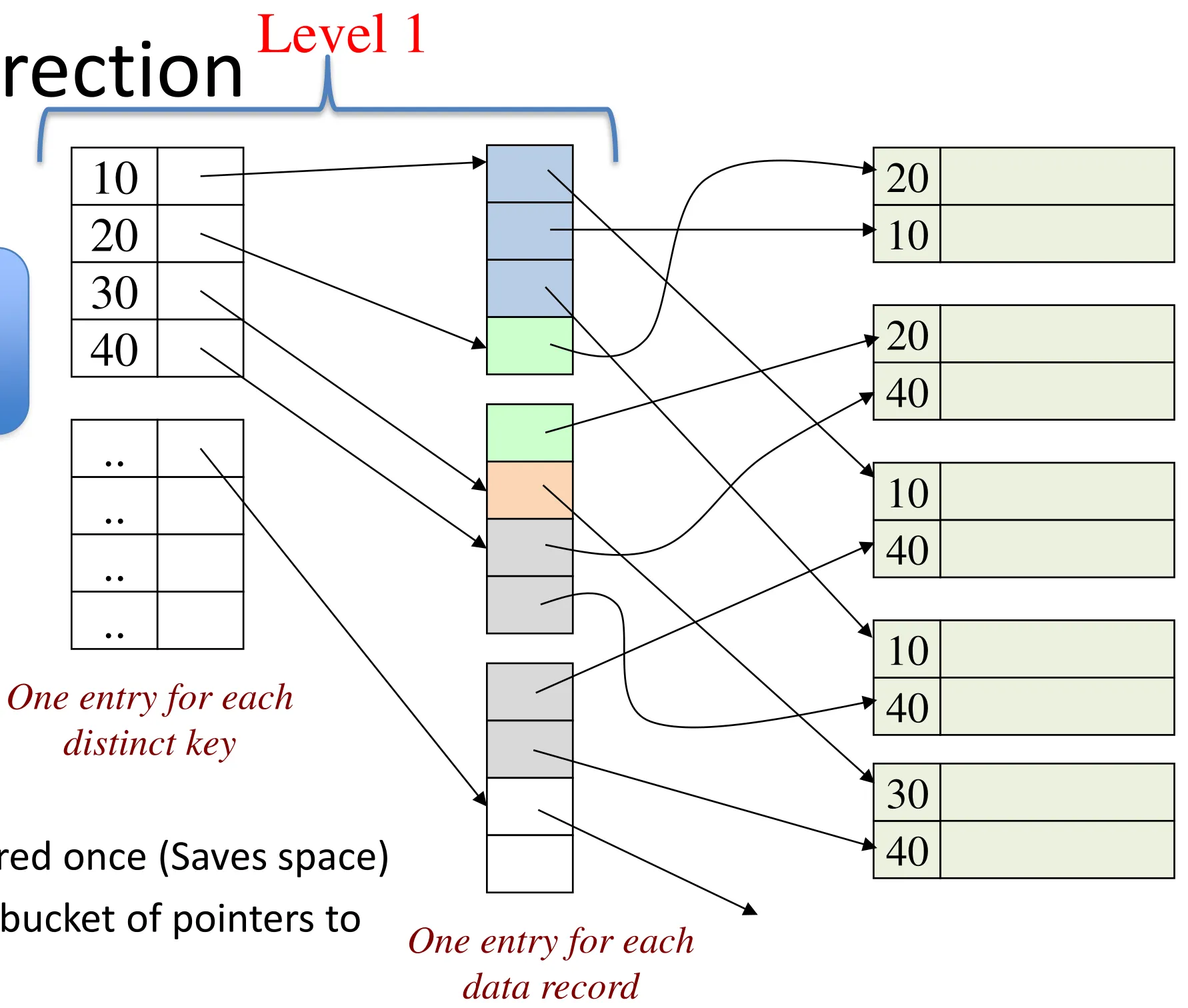
• Option 2: indirection

  • Build a 2nd level index to store distinct values of the key

  • Each distinct value stored once (Saves space)

  • Each value points to a bucket of pointers to the duplicate values

• B-trees

  • A disk-based multi-level balanced tree index structure

    • Disk-based

      • Each node in the tree is a disk page → has to fit in one disk page

      • The pointers are locations on disk either block ID or record ID

    • Multi-level

      • Has one root (can be the only level)

      • The height of the tree grows and shrinks dynamically as needed

      • We always (in search, insert, delete) start from the root and move down one level at a time

    • Balanced

      • All leaf nodes are at the same height

  • B+ tree

    • Self-balancing, ordered tree data structure that allows searches, sequential access, insertions, and deletions in O(log n)

      • Generalization of a binary search tree, since a node can have more than two children

      • Optimized for systems that read and write large blocks of data

  • Properties

    • Each node (which is disk block) holds N keys and N + 1 pointers

    • Keys in any node are sorted from left to right

    • Keys in any level are also sorted from left to right

    • Each node is at least 50% full (Minimum 50% occupancy)

      • Except the Root can have as minimum (1 key & 2 pointers)

    • No empty spaces in the middle of a node

    • Number of pointers in any node = number of keys + 1

      • The rest are Null

  • Leaf node values

    • Approach #1: Record IDs

      • A pointer to the location of the tuple to which the index entry corresponds

    • Approach #2: Tuple Data

      • The leaf nodes store the actual contents of the tuple

      • Secondary indexes must store the Record ID as their values

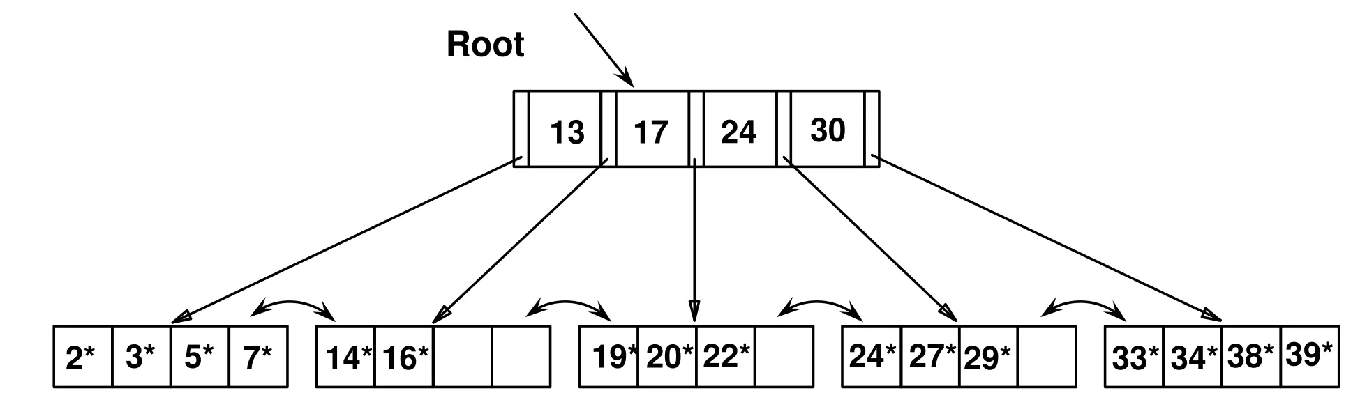
  • B+ tree visualization

• Good utilization

  • B-tree nodes should not be too empty

  • Each node is at least 50% full (Minimum 50% occupancy)

    • Except the Root can have as minimum (1 key & 2 pointers)

  • Use at least

    • Non-leaf: ceil((n+1)/2) pointers

    • Leaf: floor((n+1)/2) pointers to data

• B-tree vs. B+tree

  • The original B-Tree from 1972 stored keys and values in all nodes in the tree.

  • A B+ Tree only stores values in leaf nodes.

  • B+tree more space-efficient, since each key only appears once in the tree.

  • Inner nodes only guide the search process.

• Dense vs. sparse

  • In Theory, leaf level can be either dense or sparse

    • Sparse only if the data file is sorted

  • In Practice, in most DBMS the leaf level is always dense

    • One index entry for each data record

  • What about values in non-leaf levels?

    • Not necessarily a subset of leaf values

• B-tree in practice

  • Usually 3- or 4-level B-tree index is enough to index even large files

  • The height of the tree is usually very small

    • Good for searching, insertion, and deletion

    • Few I/Os (especially that the root can be always cached in memory)

• Querying

  • Equality Search: Find all records with a search-key value of k.

    • 1. Start with the root node

      • Examine the keys (use binary search) until find a pointer to follow

    • 2. Repeat until reach a leaf node

    • 3. Search keys in the leaf node for the first key = k

    • 4. Follow the pointers to the data records

  • Range Search: Find all records between [k1, k2].

    • 1. Start with the root node and search for k1

      • Examine the keys (use binary search) until find a pointer to follow

    • 2. Repeat until reach a leaf node

    • 3. Search the keys in the leaf node for the first key = k1 or the first larger

    • 4. Move right while the key is not larger than k2 (may move from one node to another node)

    • 5. Follow the pointers to the data records

• Insertion

  • Find correct leaf L (searching)

  • Put data entry onto L

    • If L has enough space, done

    • Else, must split leaf node L (into L and a new node Lnew)

      • Redistribute entries evenly

      • Copy up middle key (1st value in LNEW) to parent.

      • Insert index entry pointing to LNEW into parent of L.

  • This can happen recursively

    • To split internal node, redistribute entries evenly, but push up middle key. (Contrast with leaf splits.)

  • Splits “grow” tree; root split increases height.

    • Tree growth: gets wider or one level taller at top.

• Deletion

  • Start at root, find leaf L where entry belongs. (Searching)

  • Remove the entry.

    • If L is at least half-full, done!

      • Do not leave empty spaces in the middle

    • If L has less than the minimum entries,

      • Try to re-distribute, borrowing from sibling (adjacent node with same parent as L).

      • If re-distribution fails, merge L and sibling.

  • If merge occurred, must delete entry (pointing to L or sibling) from parent of L.

  • Merge could propagate to root, decreasing height.

• More practical deletion

  • When deleting 24*, allow its node to be under utilized

  • After some time with more insertions

    • Most probably more entries will be added to this node

  • If many nodes become under-utilized ➔ Re-build the index

• Hashing

  • Static hashing

    • Disk-based hash-based indexes

      • Adaptation of main memory hash tables

      • Support equality searches

      • No range searches

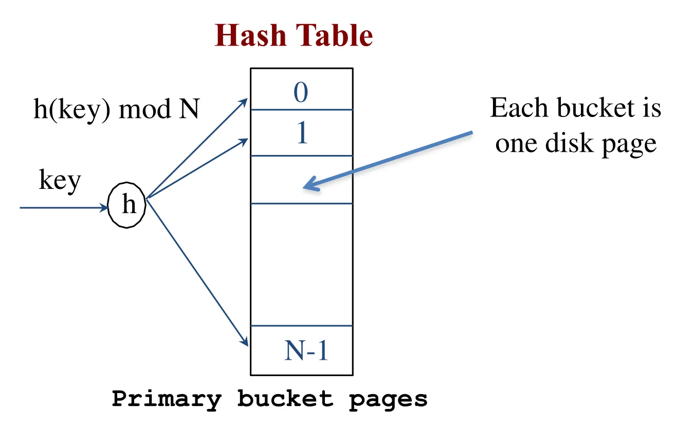
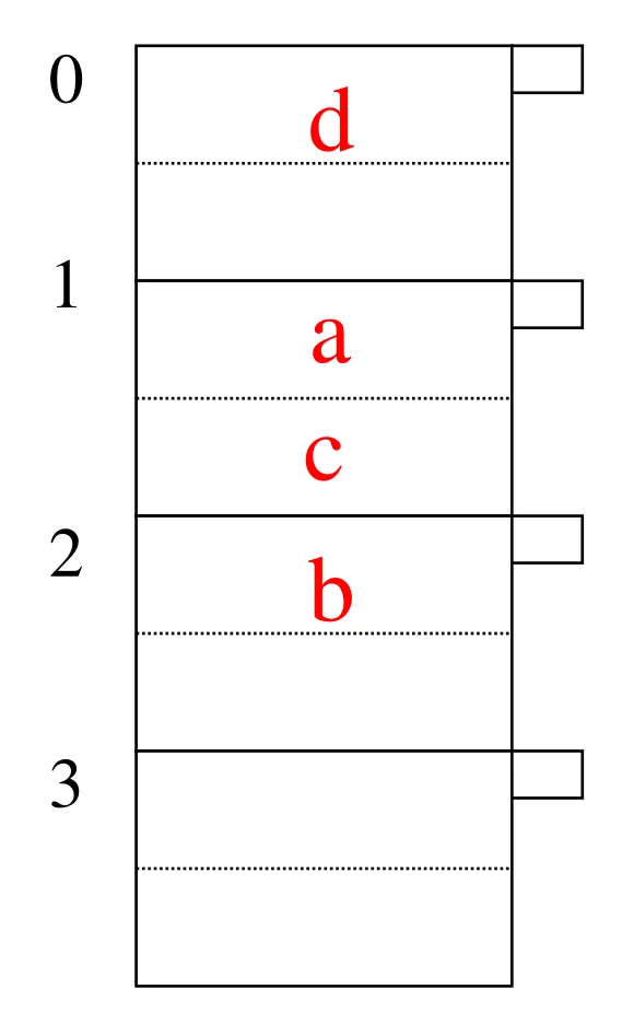
    • Hash table has N buckets (static means “N” does not change

      • Each bucket will be one disk page

      • Hash function h(k) maps key k to one of the buckets

• Within a bucket

• Should we keep entries sorted?

  • Yes, if we care about CPU time

  • Makes the insertion and deletion a bit more expensive

• Lookup (Search for key = d)

  • Apply the hash function over d ➔ h(d) mod N = 0

  • Read the disk page of bucket 0

  • Search for key d

    • If keys are sorted, then search using Binary search

• Insertion

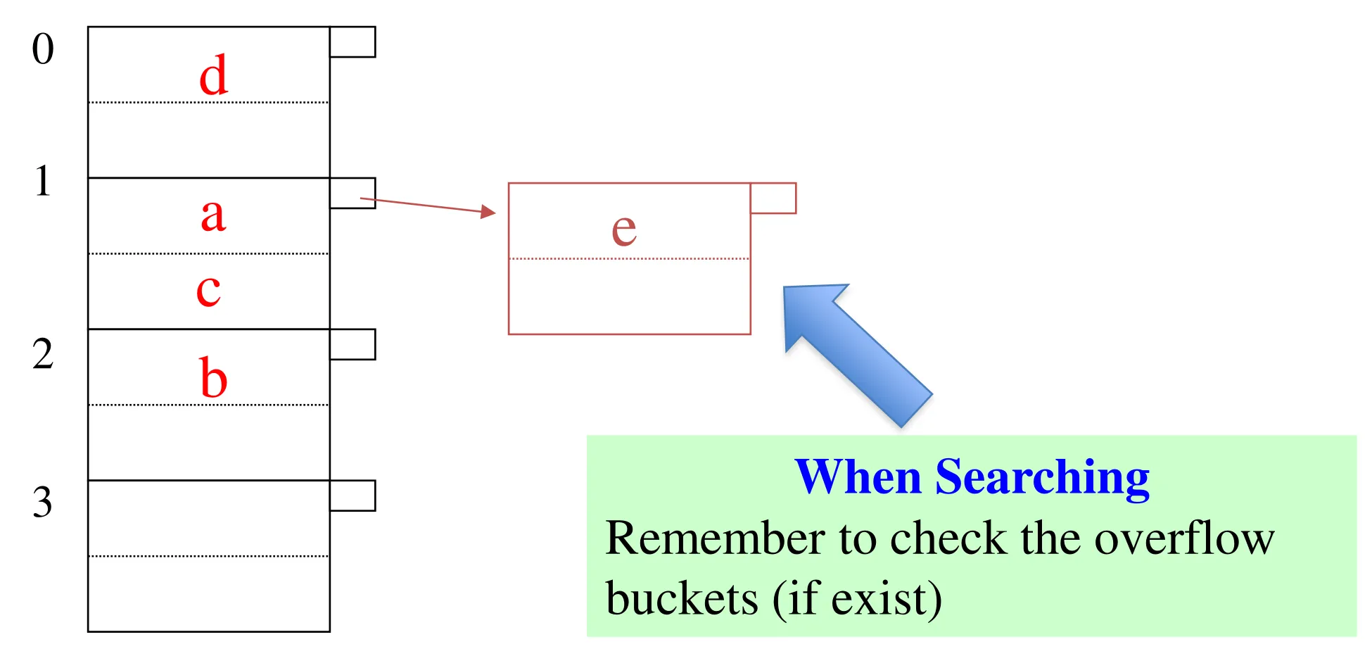
• Insertion with overflow

  • Insert key e ➔ h(e) mod N = 1

  • Create an overflow bucket and insert e

  • Overflow bucket is another disk block

• Deletion

  • Search for the key to be deleted

  • In case of overflow buckets

    • The overflow bucket may no longer be needed

• Extensible (dynamic) hashing

  • No overflow buckets

  • The number of primary buckets is not fixed and it can grow

  • Start with some # of buckets (e.g., N=4 and h(k) = k)

  • Each bucket can fit fixed # of entries (e.g., M=4)

  • Problem: storing index entries directly on primary bucket eventually requires overflow buckets

  • Solution: Rather than storing entries directly, use a directory

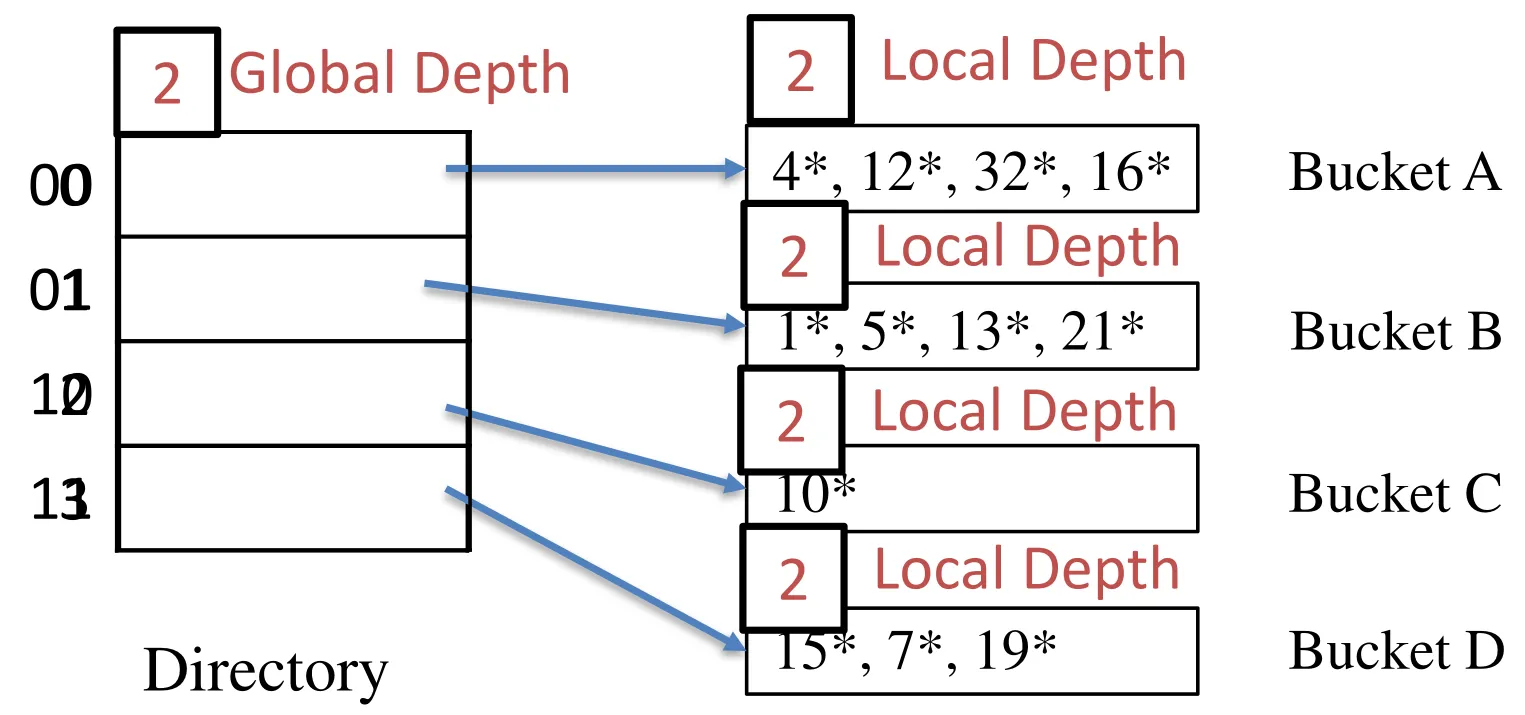
  • Binary representation (N=4)

    • Here we can use 2 bits to represent buckets (global depth=2)

    • How can we find bucket for key 12?

      • Look at 2 rightmost bits of h(12)

    • Every key in bucket A has the same 2 last bits (local depth=2)

      • Same for others

• Given a key k ➔ we need to know k will go to which entry in the directory

• Hash Function

  • Convert k into binary representation (0s and 1s)

  • Consider only the number of bits equal to the Global Depth value

    • Take bits from right side (Least Significant bits)

• Insertion

  • Case 1: Expand under local depth = global depth

    • Increment global depth

    • This means ➔ double the directory size

    • For the overflow bucket, divide into two

    • Increment their local depth

    • Re-distribute the keys based on the new local depth bits

    • For all other buckets, leave them as is (local depth < global depth)

    • Number of incoming pointers to each of these bucket is doubled

  • Case 2: Split while local depth < global depth

    • No need to double Directory

    • Only split the bucket

    • Increment local depth

    • Re-distribute its keys

• SQL & Query Processing

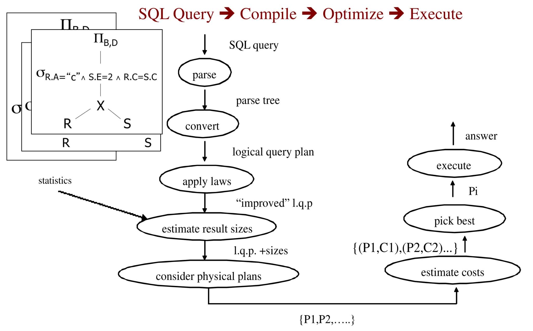
  • Execution engine

    • Receives query plan from the query compiler and executes

  • Relational algrebra express query plans

    • Intuition

      • Avoid cross product

      • Push down unary operators

      • Perform joins on smaller datasets

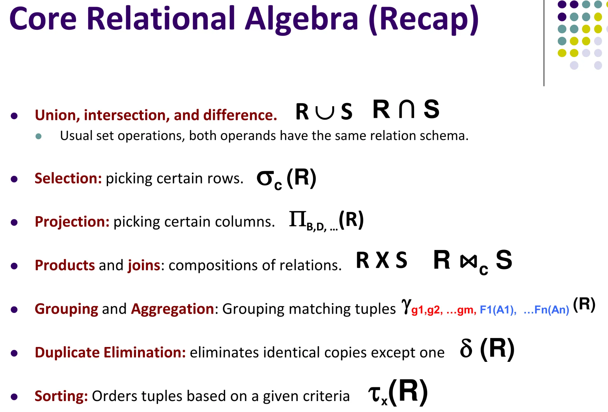
• Set of operators that operate on relations

• Operator semantics based on Set or Bag theory

• Relational algebra form underlying basis (and optimization rules) for SQL

• Query planning

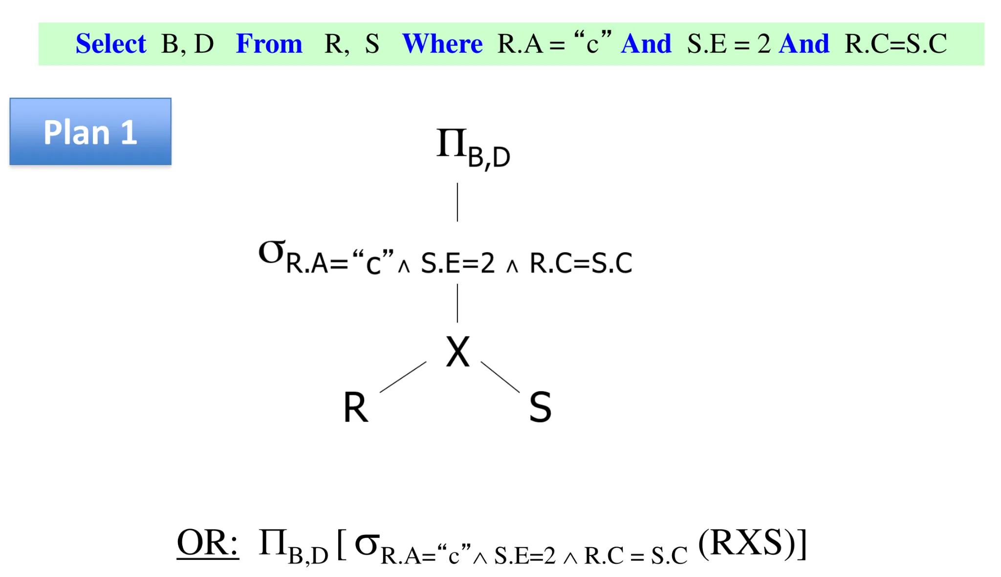
  • Goal: equivalent query plans but cheaper operationally

  • Intuition

    • Minimize the size (number of tuples, number of attributes) of intermediate results

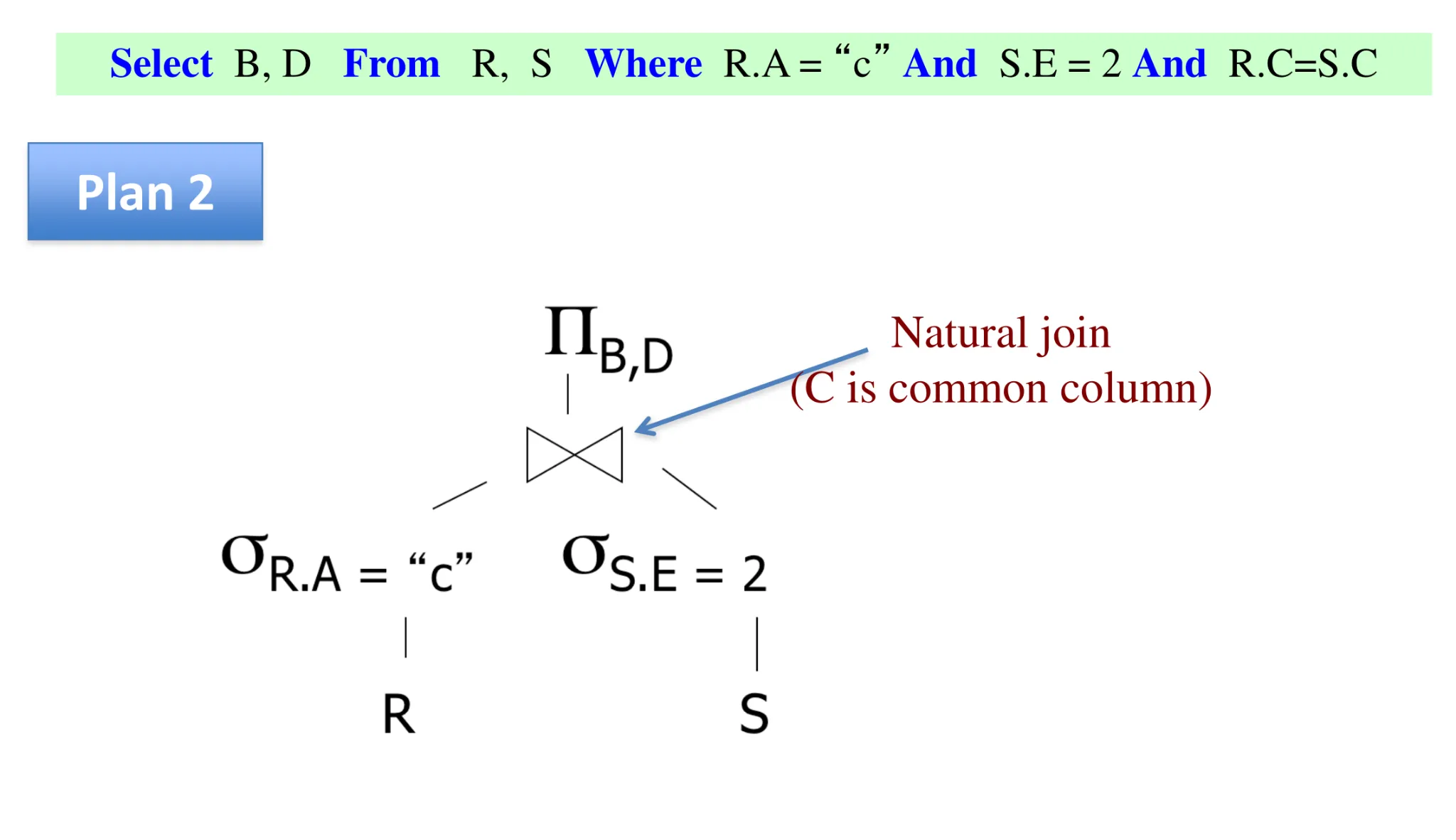
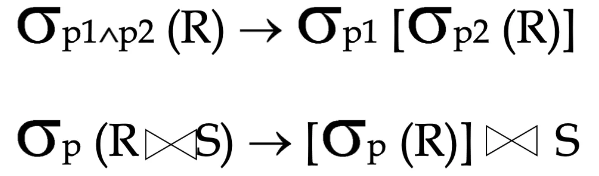
    • Push selections down in the expression tree as far as possible

    • Push down projections, or add new projections where applicable

• Overview of query execution

• Heuristics

  • Pushing selections

• Dhisfo

  • Replace the left side of one of these (and similar) rules by the right side

  • Can greatly reduce number of tuples in intermediate results

  • Operator evaluation

    • Two categorizations

      • Technique

      • Number of passes

    • Algorithms for evaluating relational operators use some simple ideas extensively:

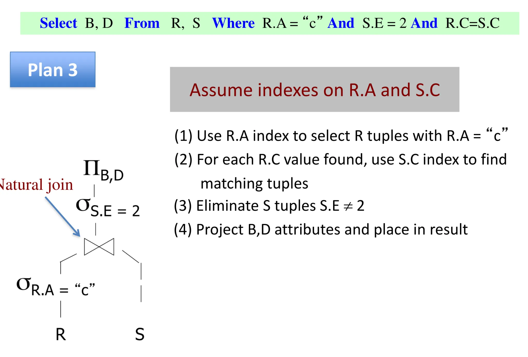
      • Indexing: Can use WHERE conditions to retrieve small set of tuples (selections, joins)

      • Iteration: Sometimes, faster to scan all tuples even if there is an index. (Sometimes we can scan the data entries in an index instead of the table itself (when?)

      • Partitioning: By using sorting or hashing, we can partition the input tuples and replace an expensive operation by similar operations on smaller inputs.

    • Number of passes: 1 pass, 2 pass, multi-pass

  • Common statistics over relation R

    • M: # of memory buffers available

    • B(R): # of blocks to hold all R tuples

    • T(R): # tuples in R

    • S(R): # of bytes in each of R’s tuple

    • V(R, A): # distinct values in attribute R.A

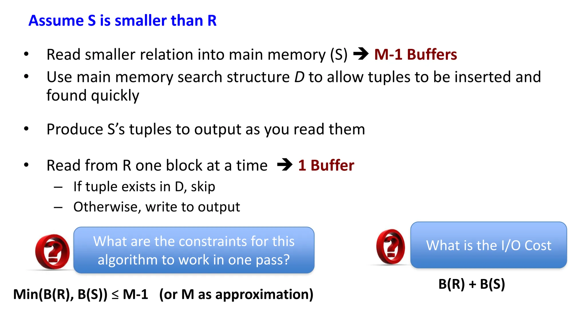
  • One pass operator evaluation algorithms

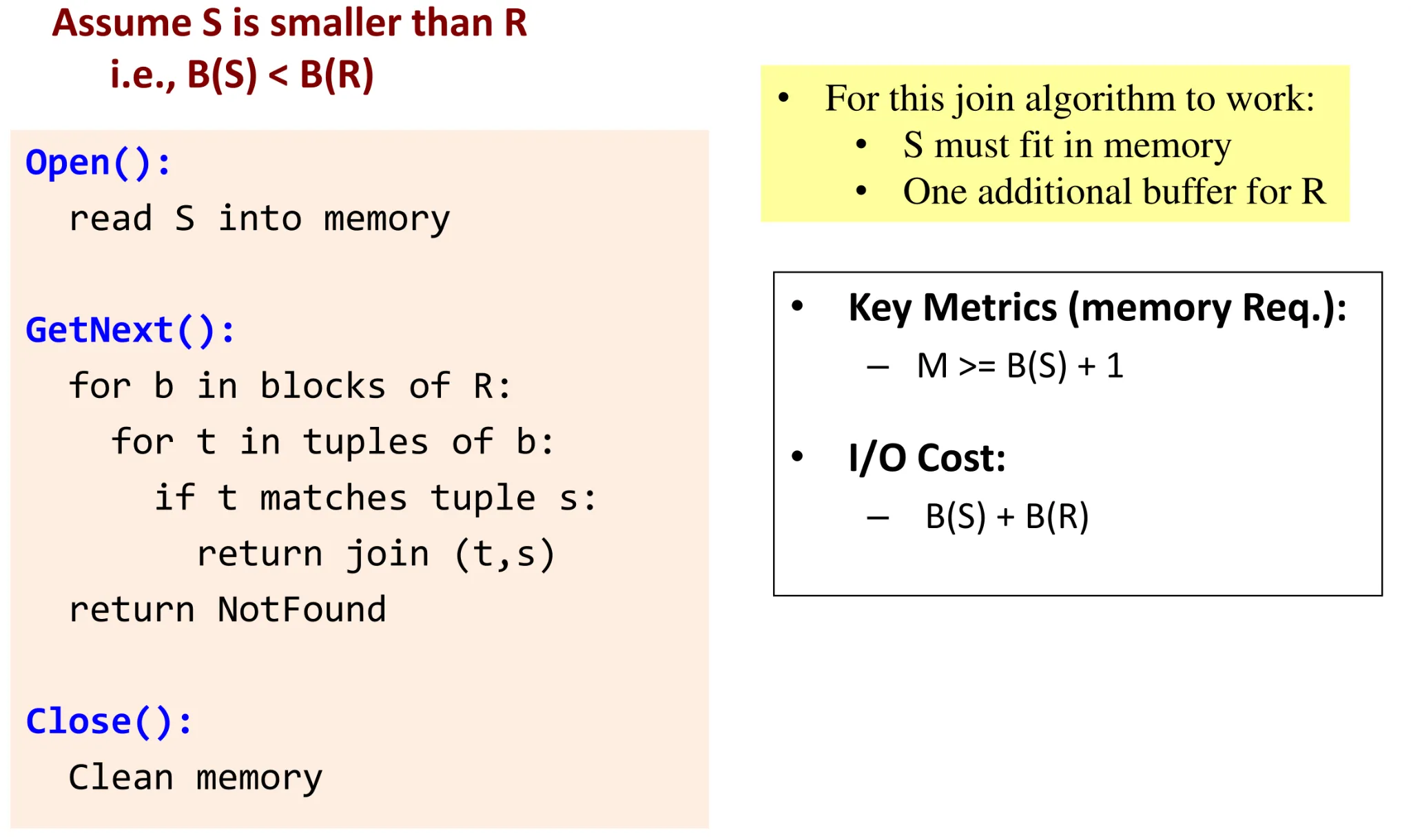
    • Join (R, S)

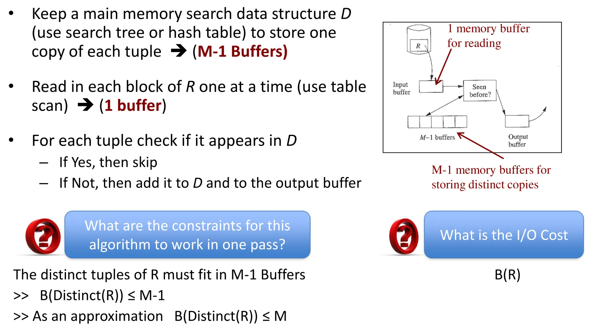
• Duplicate elimination

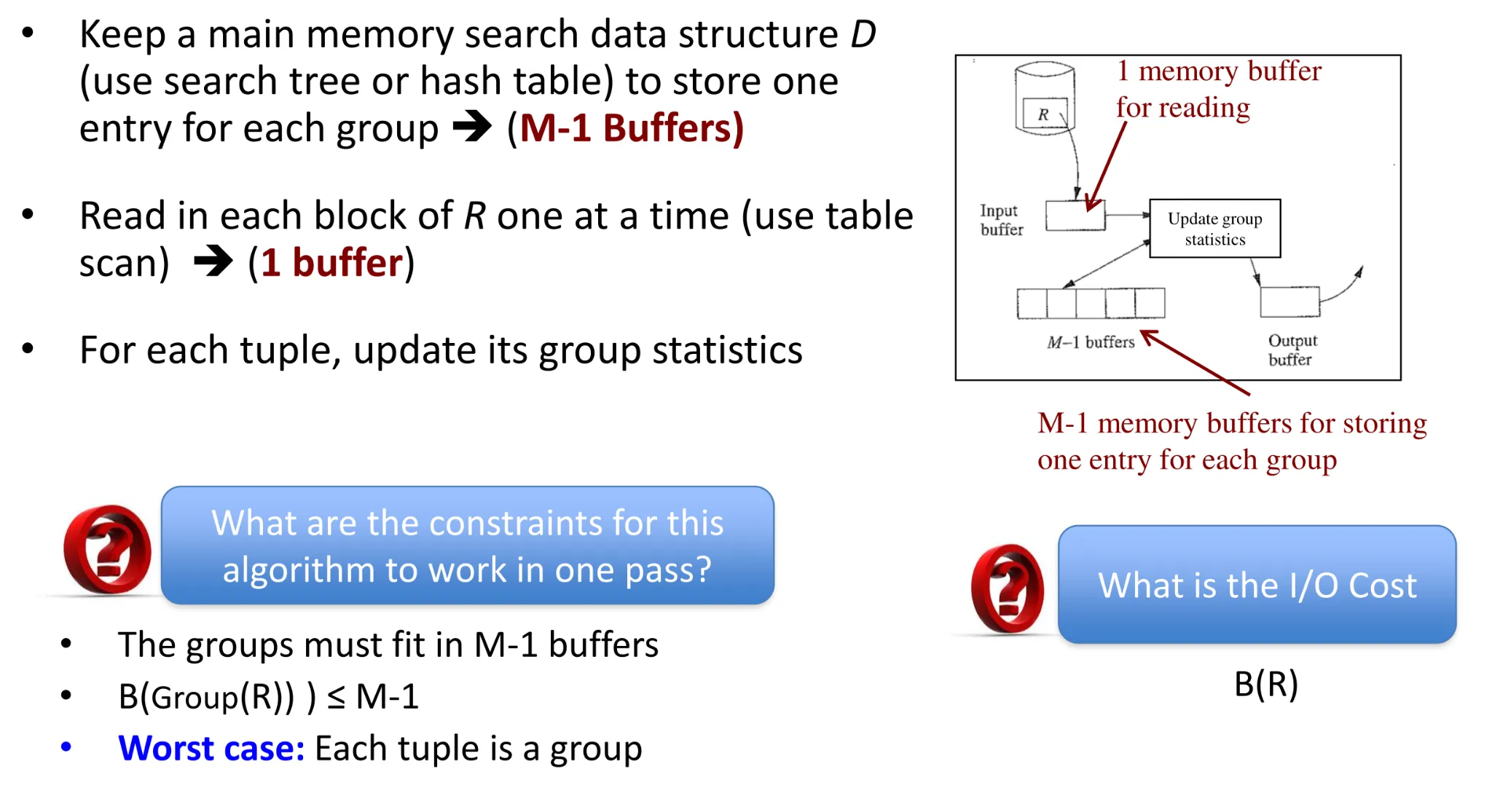
• Group by

• Set union(R,S)

• Blocking vs. non-blocking operators

  • Blocking operator cannot produce any tuples to the output until it processes all its inputs

  • Non-blocking operator (Pipelined) can produce tuples to output without waiting until all input is consumed

  • Examples

    • Join, duplicate elimination, union ➔ Non-blocking

    • Grouping ➔ Blocking

    • Selection, Projection ➔ Non-blocking

    • Sorting ➔ Blocking

• Two pass algorithms

  • First Pass: Do a prep-pass and write the intermediate result back to disk

    • We count Reading + Writing

  • Second Pass: Read from disk and compute the final results

    • We count Reading only (if it is the final pass)

  • Sort-based two-pass algorithms

    • 1st pass does a sort on some parameter(s) of each operand

    • 2nd pass algorithm relies on sort results; can be pipelined

  • Hash-based two-pass algorithms

    • 1st pass partitions input relation

    • 2nd pass algorithm will work on each partition independently

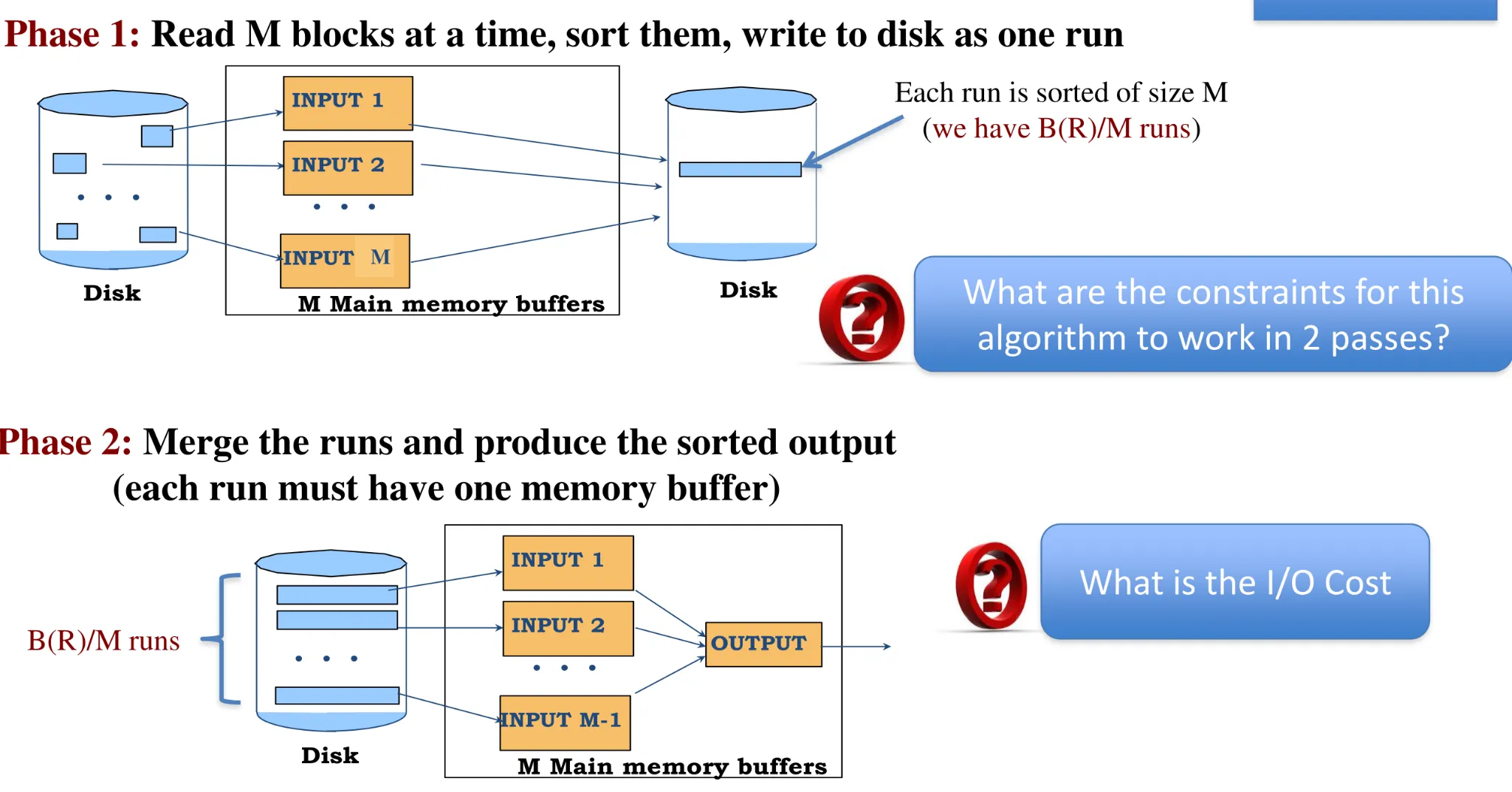
  • 2-Pass external sort

• Phase 1 → no constraints

• Phase 2 → each run must have a memory buffer + one for output

• B(R)/M ≤ M-1

• Approx. B(R)/M ≤ M

• B(R) ≤ M^2