CS 3431: Database Systems I
- Terminology
- Database
- Collection of information that exists over a long period of time
- DBMS
- Software platform that allows us to create, store, use, and maintain a database
- Allows users to create new DBs and specify their schemas (logical structure of the data), using a specialized DDL
- Allows users to query and modify the data using DML
- Supports the storage and efficient access to very large amounts of data
- Enables durability, the recovery of the DB in case of failures
- Control access to data from many users at once, without allowing unexpected interactions among users (called isolation) and without actions on the data to be performed partially but not completely (called atomicity).
- Frontend
- Data Definition Language - DDL
- Data Manipulation Language - DML
- Backend
- Query compiler
- Query engine
- Storage management
- Transaction management (concurrency, recovery)
- Model
- Tools used for describing the data
- Schema
- Describes structures for a particular application using the given model
- Database
- Collection of actual data that conforms to the given schema
- SQL & Data Manipulation Language
- Language to manipulate (update or query) the data
- Database
- Why use DBMS, and not files?
- Data redundancy and inconsistency
- Difficulty in accessing data
- Integrity problems
- Maintenance problems
- Concurrent access by multiple users
- Security problems
- Recovery from crashes
- A simple client/server system
- The computer server is running DB software that provides services to client software
- Client software accessing the DB can even reside on the DB server
- Clients send SQL queries and the DB server sends back the results
- Results are transmitted over a network → Important to write efficient queries
- Overview of a DBMS
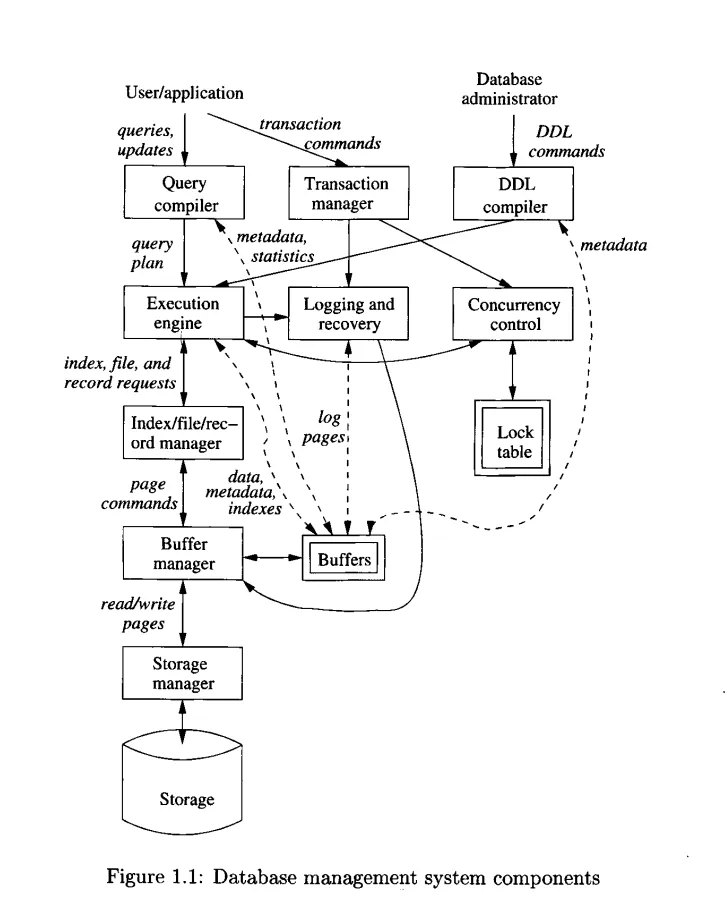
Single boxes represent system components, while double boxes represent in-memory data structures. The solid lines indicate control and data flow, while dashed lines indicate data flow only.
- Two distinct sources of commands to the DBMS
- Conventional users and application programs that ask for data or modify data.
- A database administrator: a person or persons responsible for the structure or schema of the database
- DDL commands
- DDL commands by a DB admin are parsed by a DDL processor and passed to the execution engine, which then goes through the index/file/record manager to alter the metadata (the schema information for the DB)
- Overview of query processing
- DML commands do not affect the DB schema but may affect the content of the DB or extract data from the DB
- DML statements are handled by two separate subsystems
- Queries — single requests for data from the DB
- Queries don’t have to pass through the transaction manager because they can be executed independently. If you are simply retrieving data from the database, there is no need to use a transaction.
- Queries are parsed and optimized by a query compiler → query plan (sequence of actions the DBMS will perform to answer the query)
- Query plan is passed to the execution engine, which issues a sequence of
requests for small pieces of data (records or tuples of a relation) to a
resource manager
- The resource manager knows about data files (holding relations), the format and size of records in those files, and index files, which help find elements of data files quickly
- The requests for data are passed to the buffer manager
- The buffer manager brings appropriate portions of the data from secondary storage (disk) where it is kept permanently to the main memory buffer
- The page/“disk block” is the unit of transfer between buffers and disk
- The buffer manager communicates with a storage manager to get data from
disk
- The storage manager might involve OS commands, but more typically, the DBMS issues commands directly to the disk controller
- Transaction (group of queries and other DML actions) processing
- Unlike queries, if you are modifying data in the database, it is generally a good idea to use a transaction to ensure the integrity of the data
- Units that must be executed atomically, in isolation from one another, and durable (effects preserved even if the system fails after the completion of the transaction)
- Transaction commands are passed to the transaction manager which has two
parts
- A concurrency-control manager, or scheduler, responsible for assuring atomicity and isolation of transactions
- A logging and recovery manager, responsible for the durability of transactions
- Queries — single requests for data from the DB
- Storage and buffer management
- The data of a DB mainly resides in secondary storage (disk)
- To perform useful operation on data, that data must be in main memory
- The storage manager
- Controls the placement of data on disk and its movement between disk and main memory
- Keeps track of the location of files on the disk
- Obtains a block/blocks containing a file on request from the buffer manager
- The buffer manager
- Partitions the available main memory into buffers, which are page-sized regions into which disk blocks can be transferred
- All DBMS components that need information from the disk will interact with
the buffers and the buffer manager. Different types of information include
- Data: the contents of the DB itself
- Metadata: the database schema that describes the structure of, and constraints on, the database.
- Log Records: information about recent changes to the database; these support the durability of the database.
- Statistics: information gathered and stored by the DBMS about data properties such as the sizes of, and values in, various relations or other components of the database.
- Indexes: data structures that support efficient access to the data
- In a simple DBMS, the storage manager can be the file system itself (SQLite)
- Normally, DMBS controls storage on the disk directly
- Transaction processing
- The transaction manager accepts transaction commands from an application, which tells the beginning and end of a transaction
- The transaction manger then performs
- Logging
- Every change in the DB is logged separately on disk
- The log manager follows a policy to assure that when a crash occurs, a recovery manager will examine the log of changes and restore the DB to a consistent state
- The log manager writes the log in buffers initially and negotiates with the buffer manager to make sure that buffers are written to the disk (survive crashes) at appropriate times
- Concurrency control
- Assure the net effect of multiple transactions executed at once is the same as if the transactions had executed one-at-a-time
- The scheduler does this by maintaining locks on certain pieces of the DB, these prevent two transactions from accessing the same piece of data in ways that interact badly
- Locks are stored in a main memory lock table
- The scheduler forbids the execution engine from accessing locked parts of the database
- Deadlock resolution
- Transactions can sometimes have circular dependency
- The transaction manager has to intervene and roll back or abort one or more transactions to let others proceed
- Logging
- The query processor
- Has two components - Query compiler - Translates the query into an internal form called a query plan - The operations in a query plan are implementations of relational algebra operations - The query compiler consists of three major units - Query parser — builds a tree structure from the textual form of the query - Query preprocessor — performs semantic checks on the query and performs tree transformations, turning the parse tree into a tree of algebraic operators representing the initial query plan - Query optimizer — transforms the initial query plan into the best available sequence of operations on the actual data - Execution engine - Executes each step in the chosen query plan - Gets data from the DB into buffers to manipulate - Interacts with the scheduler to avoid accessing locked data - Interacts with the log manager to make sure that all DB changes are properly logged
- The ACID properties of transactions
- Properly implemented transactions meet the ACID test
- Atomicity — all-or-nothing execution of transactions
- Consistency — transactions preserve the consistency of the database
- DBs have consistency constraints (non-negative account balances)
- Isolation — transaction must appear to execute as if no other transaction is executing at the same time
- Durability — the effect of the transaction on the DB must never be lost, once the transaction has been completed
- Properly implemented transactions meet the ACID test
- Data Model
- A collection of tools for describing
- Data objects
- Data relationships
- Data semantics
- Data constraints
- Several data models
- Relational model
- Entity-Relationship (ER) data model
- Semi-structured data model (XML)
- Object-based data models (Object-oriented)
- Other older models
- Network model
- Hierarchical model
- A collection of tools for describing
- Data Schema
- Captures the relationships between objects (entities) in an application
- Schemas can be represented graphically or textually
- Query Language
- Language for accessing and manipulating the data organized by the appropriate data model
- Levels of abstraction
- View level — describes how users see the data
- Logical level — describes the logical structures used
- Relational model
- ER model
- Physical level — describes files and indexes
- These levels lead to data independence
- Physical data independence
- Physical schema such as indexes can change, but logical schema do not need to change
- Protection from changes in physical structure of data
- Logical data independence
- Logical schema can change, but views do not need to change
- Protection from changes in logical structure of data
- Physical data independence
- Relational Data Model
- The most widely used model today
- Tabular representation of the data
- Main concepts
- Relations (tables) are tables with rows and columns
- Every relation has a schema, which describes the columns, or fields
- The Entity-Relationship Data Model
- Models the application as a collection of entities and relationships
- Represented using Entity-Relationship Diagram (ERD)
- DB Design stages
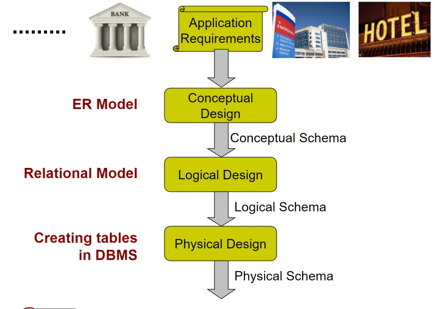
- Conceptual design
- ER Model
- Structures: Entities and Relationships
- Constraints
- ER Model
- Modeling
- A DB can be modeled as
- Collection of entities
- Relationship among entities
- An entity is an object that exists and is distinguishable from other objects
- Entities have attributes — property of an entity, has a domain
- A relationship is an association (connection) between entities
- May have attributes — do not belong to connected entities, belong to the relationship
- A DB can be modeled as
- ERD representation
- Entity set — rectangle
- Attribute — oval
- Relationship — diamond
- Attribute types
- Primitive attributes: Attribute stores a single value (Number, String, Boolean, Date, …)
- Composite attributes: An attribute can be divided into sub-attributes (each is primitive)
- Multi-values attributes: Attribute with many values
- Derived attributes: Attributes computed from others
- Relationship types
- Binary
- Ternary
- Multi-way
- Recursive (must have roles)
- Weak
- ISA
- Key constraints
- Key of entity set is the set of attributes that uniquely identify each identity
- A key has to be unique within the scope of your application
- Does not have to be globally unique
- Types of keys
- Super key is a set of one or more attributes whose values uniquely determine each entity
- Candidate key (minimal super key)
- Each candidate key is a super key but not vice versa
- Primary key (any one from the candidate keys)
- Only primary keys are modeled in ERD by underlining an entity’s set of
attributes
- Good practice: select singleton and number attributes whenever possible
- Keys of relationships
- Relationship without attributes
- Combination of primary keys of the participating entity sets forms a key of a relationship set
- Relationship with attributes
- Attributes of the relationship may (not always) participate inside the key + the external keys
- Relationship without attributes
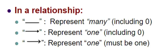
- Cardinality constraints
- Express the number of entities to which another entity can be associated via a relationship set
- Most useful in describing binary relationship sets
- For a binary relationship set the mapping cardinality must be one of the
following types:
- One to one
- One to many
- Many to one
- Many to many
- Express the degree of cardinalities using (min, max)
- Adding degree constraints over multi-way relationships is
- complex and not easy to understand
- To add degree constraints, introduce a new entity set and create multiple binary relationships
- Weak entities
- Is an entity set that does not have a primary key
- Its attributes are not enough to form a key
- The existence of a weak entity set depends on the existence of an
identifying entity set
- It must relate to the identifying entity set via a total, one-to-many relationship set from the identifying to the weak entity set
- Discriminator (partial key)
- The set of attributes that uniquely identify a weak entity given its identifying entity
- Primary key of a weak entity set
- The composition of the primary key of the identifying entity set + the weak entity set’s discriminator
- An identifying entity has to exist for each weak entity
- Representation
- Weak entity sets are represented by double rectangles
- Weak relationship (supporting relationship) is represented by double diamonds
- Weak relationship is one-many
- Is an entity set that does not have a primary key
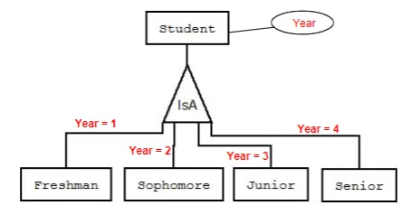
- Subclass entities (ISA relationships)
- Similar to subclass concepts in OOP
- Entity sets share some common attributes but differ in others
- All attributes and relationship participation of the parent entity set are inherited in all children entity sets
- Each child entity set can have its own additional attributes and relationship participation
- Keys of sub-entities are inherited from the super entities
- Constraints
- Membership: Constraint on which entities can be members of a given
lower-level entity set
- Denoted in ERD on the ISA edge
- Membership: Constraint on which entities can be members of a given
lower-level entity set
- Overlapping: Can an entity belong to multiple subclasses or not
- Disjoint
- An entity can belong to only one lower-level entity set
- Overlapping
- An entity can belong to more than one lower-level entity set
- Denoted in ERD by writing “disjoint” or “overlapping” inside the ISA triangle, by default “disjoint
- Disjoint
- Completeness: Does each super entity have to belong to one (or more)
subclasses
- Total: An entity must belong to one of the lower-level entity sets
- Partial: An entity need not belong to one of the lower-level entity sets
- Representation
- IsA relationships are represented by a triangle component labeled ISA
- Always one-to-one (even though the notation is arrows without heads)
- Principles for good design
- Convey “real” application requirements
- Utilize meaningful names for entity sets, attributes, relationships
- Avoid redundancy, do not store the same data in multiple places
- Be as precise as possible (E.g., cardinality constraints)
- Don’t over specify (limits input)
- Know when to add attributes to entity sets vs. relationships
- M-M Relationship between E1 and E2 can be always broken to:
- A new entity set E3 (usually weak entity set)
- 1-M relationship between E1 and E3
- 1-M relationship between E2 and E3
- Do not overuse ISA relationship
- There are always some commonalities between things this does not mean they should inherit from common ancestor
- Use it only if there is a substantial overlap in attributes (and possibly relationships)
- Strong vs. Weak Entity Sets
- Avoiding weak entities is better (If no semantics is lost)
- You may add unique keys
- Do not overuse multi-way relationships
- They are harder to understand and interpret
- Can be broken by introducing a new entity set and several 1-M relationships
- ERD cannot capture everything - Some business constraints will not be captured in the design. For example: - For a customer to get a loan, the sum of the previous loans to him/her must be < MaxLoan - A student cannot take the same course more than 2 times - A student cannot re-take a course that they already passed -
- Convey “real” application requirements
- Relational model
- Another model for describing your data and application requirements
- Currently the most widely used model
- Structures
- Relations (tables)
- Attributes (columns/fields)
- Tuples (rows)
- Attributes
- Each attribute of a relation has a unique name within the relation
- The set of allowed values for each attribute is called the domain of the attribute
- Attribute values are required to be atomic (primitive or derived)
- Multivalued and composite attributes are not atomic
- The special value NULL is a member of every domain → means that the value does not exist
- Relational schema
- Schema is the structure of the relation
- Attributes A1, A2,…, An of relation R
- R=(A1, A2,…, An) is the schema of relation R
- Relational instance
- A relational instance is the current schema plus the current tuples in the relation
- The current instance of “customer” has four tuples (rows or records)
- Instances are frequently changing
- E.g., inserting new tuples, deleting or updating existing tuples
- Schemas may also change but not frequently
- Arity & cardinality of relations
- The arity (degree) of a relation
- Number of attributes of that relation
- Cardinality of a relation
- Number of tuples in that relation
- The arity (degree) of a relation
- Relations are unordered
- The order of tuples is not important
- The order of columns is not important
- Think of a relation as a set (or bag) of tuples not as a list of tuples
- Most current DBMSs allow bags
- Keys of relations
- Super Keys
- Subset of attributes that uniquely identify each tuple
- Candidate Keys
- Minimal super key
- Primary Keys
- Choose any of the candidate keys
- Represented by “underline” under the selected attributes
- Set vs. Bag
- If a relation has a primary key, then it is a set, not a bag
- Super Keys
- Create relations with SQL
- Data Definition Language (DDL)
- Create tables, specifying the columns and their types of columns, the primary keys, etc.
- Drop tables, add/drop columns, add/drop constraints — primary key, unique, etc.
- Data Manipulation Language (DML)
- Update, Insert, Delete tuples
- Query the data
- Data Definition Language (DDL)
- Domain types in SQL
- String data
- char(n): Fixed length character string, with user-specified length n
- varchar2(n): Variable length character strings, with user-specified maximum length n
- Numbers:
- int: Integer
- real: floating point number
- number(p,s): Number with precision p and scale s
- Boolean:
- Make it char(1) [Y/N or T/F], or number(1) [1/0]
- Date & Time:
- Date: Date field with certain format
- Timestamp: Date plus time with a certain format
- String data
- Dropping & altering tables
- Dropping (Deleting) a table
- DROP TABLE <tableName>;
- Altering a table to add a column
- ALTER TABLE <tableName> ADD <col> <type>;
- The initial value of the column is Null
- Altering a table to drop a column
- ALTER TABLE <tableName> DROP COLUMN <col>;
- Some DBMSs do not support dropping columns
- Dropping (Deleting) a table
- Integrity constraints
- Conditions that must be True for any instance of the DB
- Specified when the schema is defined
- Checked when relations are modified
- A legal instance of a relation satisfies all specified ICs.
- DBMS should not allow illegal instances
- Key constraints
- Primary Key
- Each relation may have only one PK
- Do not accept NULL
- Unique (other candidate keys)
- Each relation may have possibly many unique keys
- Accept NULL
- Primary Key
- NOT NULL & DEFAULT constraint types
- Domain values constraint with CHECK
- Foreign key constraints (referential integrity)
- Set of fields in one relation that refers to a tuple in another relation
- FK in referencing relation must match PK of referenced relation
- Match = same number of columns, compatible data types (column names can be different)
- The relationship is many-to-one from the “referencing” to the “referenced”
- DBMS will prevent FK values that do not exist in the PK column(s)
- If the referenced tuple is deleted
- CASCADING — also delete all tuples that refer to it
- NO ACTION — disallow deletion of the referencing tuple since there are dependent tuples
- SET DEFAULT — set FK in referencing tuples to a default value
- SET NULL — set FK in referencing tuples to NULL (not always applicable)
- Conditions that must be True for any instance of the DB
- DML
- Insertion (entire record)
- Insert into Students values (‘1111’, …);
- Deletion (entire record)
- Delete from Students; //delete all students
- Delete from Students Where sid = ‘53666’;
- Update (some attributes)
- Update Students Set GPA = GPA + 0.4; //update all
- Update Students Set GPA = GPA + 0.4 Where name = ‘Smith’;
- Insertion (entire record)
- Translating ER Diagrams to Relational Model
- PKs allow entity sets and relationship sets to be expressed uniformly as relational schemas
- Generally, each relational schema will have
- Number of columns corresponding to the number of attributes in ERD
- Column names that correspond to the attribute names
- Basic rule for mapping
- Each entity set → separate relation
- Relationships
- Many-to-many → always separate relation
- Others (one-to-many & one-to-one)
- If contributes with a key → map to separate relations
- If not → is not mapped to separate relations
- Rule 1: One-to-many & many-to-one cardinalities
- PK of the “one” side moves to the “many” side
- This transferred primary key becomes a foreign key
- The relationship itself is not mapped to a table
- Any attributes on the relationship go to the “many” side
- Rule 2: One-to-one cardinalities
- PK of either sides go to the other side
- This transferred PK becomes a foreign key
- The relationship itself is not mapped to the relational model
- Any attributes on the relationship go to the side receiving the transferred PK
- Rule 3: Many-to-many relationship
- Each entity set maps to a relation
- The relationship also maps to a relation
- Key of relationship = keys coming from both sides + any key of the relationship itself
- Rule 4: Weak entity sets
- Weak entity set does not have its own key
- It must relate to the identifying entity set via a total, one-to-many relationship set from the identifying to the weak entity set
- A weak entity set is mapped to a relation with all its attributes + the key(s) of the identifying entity set(s)
- The supporting relationship is not mapped
- PK of the new relation is the
- Identifying key(s) from identifying entity set(s), and
- Discriminator of the weak entity set
- Rule 5: Composite & Derived Attributes
- Composite: Include only the 2nd level attributes
- Derived: Mapped as is (enforced later using triggers)
- Rule 6: Multi-valued Attributes
- Becomes a relation by itself
- The PK of that relation = Attribute + the PK of the main entity set
- Rule 7: ISA relationships
- ISA is a one-to-one relationship BUT the sub-class entity sets inherit
attributes from the super-class entity set
- That is why it does not follow the one-to-one rules
- Many ways for the mapping depending on whether it is total vs. partial and overlapping vs. disjoint
- Super-class key is always the PK
- Method 1: One relation for all
- Recommended if sub-entity sets do not have many attributes or relationships of their own
- Method 2: Relations only for sub-classes
- Recommended only for total & disjoint types
- Cannot be used for partial, otherwise some entities will not fit in any relation
- If the relationship is overlapping → there will be some redundancy
- Disjoint: An entity can belong to only one lower-level entity set
- Overlapping: An entity can belong to more than one lower-level entity set
- Total: An entity must belong to one of the lower-level entity sets
- Partial: An entity need not belong to one of the lower-level entity sets
- Method 3: Relation for each entity set
- ISA is a one-to-one relationship BUT the sub-class entity sets inherit
attributes from the super-class entity set
- Relational Algebra
- Set of operators that operate on relations
- Operator semantics based on Set or Bag theory
- Relational algebra form underlying basis (and optimization rules) for SQL
- Basic operators
- Set Operations (Union: ∪, Intersection: ∩, difference: — )
- Select: σ
- Project: π
- Cartesian product: x
- Rename: ρ
- More advanced operators, e.g., grouping and joins
- The operators take one or two relations as input and produce a new relation as output
- One input → unary operator, two inputs → binary operator
- Important because query compilation, optimization, and execution rely on relational algebra
- Set operators (union, intersection, difference)
- Defined only for union-compatible relations
- Relations are union compatible if and only if
- They have the same sets of attributes (schema), and
- The same types (domains) of attributes
- Select: σc (R) (sigma)
- c is a condition on R’s attributes
- Select a subset of tuples from R that satisfy selection condition c
- Project: π → Package your results in a different way (pi)
- πA1, A2, …, An (R), with A1, A2, …, An attributes AR
- returns all tuples in R, but only columns A1, A2, …, An
- A1, A2, …, An are called Projection List
- πA1, A2, …, An (R), with A1, A2, …, An attributes AR
- Cross product (Cartesian product): x
- Number of columns = sum of number of columns
- Number of rows = product of number of rows
- Rename: ρ (rho)
- ρS (R) changes relation name from R to S
- ρS(A1, A2, …, An) (R) also renames attributes of R to A1, A2, …, An
- Composition of operators
- Can build expressions using multiple operations
- Joins - Natural Join: R ⋈ S (Join on the common attributes) - Consider relations - R with attributes AR, and - S with attributes AS. - Let A = AR ∩ AS = {A1, A2, …, An} The common attributes - In English - Natural join R ⋈ S is a Cartesian Product R X S with equality predicates on the common attributes (Set A) - Perform Cartesian product on R and S and only project the tuples that have matching common attributes
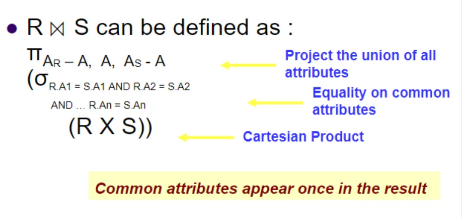
- Theta Join: R ⋈ C S
- Theta Join is cross product, with condition C
- It is defined as :
- R ⋈ C S = (σC (R X S))
- Recommendation
- Better to use Theta join (more explicit)
- Might have duplicate rows if there are common attributes in the relations
- Theta join can express both Cartesian product & natural join
- Assignment Operator: ←
- The assignment operation (←) provides a convenient way to express complex queries on multiple lines
- Write query as a sequence of lines consisting of:
- Series of assignments
- Result expression containing the final answer
- Example:
- R1 ← (σ ((A=B) ^ (D>5)) (R — S)) ∩ W
- R2 ← R1 ⋈ (R.A = T.C) T
- Result ← R1 U R2
- Duplicate Elimination: δ(R) (delta)
- Delete all duplicate records
- Convert a bag to a set
- Grouping & Aggregation operator: Ɣ (gamma)
- Aggregation function takes a collection of values and returns a single value
as a result
- avg: average value
- min: minimum value
- max: maximum value
- sum: sum of values
- count: number of values
- Grouping & Aggregate operation in relational algebra
- R is a relation or any relational-algebra expression
- g1, g2, …gm is a list of attributes on which to group (can be empty)
- Each Fi is an aggregate function applied on attribute Ai within each group
- Aggregation function takes a collection of values and returns a single value
as a result
- Relationships among operators
- Intersect as Difference
- R ∩ S = R - (R - S)
- Join as Cartesian Product + Select
- R ⋈ (C) S = σ(C)(R ⋈ S)
- Select is commutative
- σ(C2)(σ(C1)(R)) = σ(C1)(σ(C2)(R)) = σ(C1 ^ C2) (R)
- Order between Select & Project
- σ(C)(π(list)(R)) = π(list)(σ(C)(R))
- π(list)(σ(C)(R)) = σ(C)(π(list)(R)) (only if list contains all columns needed by conditions C)
- Join is commutative
- R ⋈(C) S = S ⋈(C) R
- Order between select & join
- σ(R.x = 5)(R ⋈(R.a = S.b) S) = ((σ(R.x = 5) (R)) ⋈(R.a = S.b) S)
- Intersect as Difference
- Some basic rules for algebraic expressions for better performance
- Joins vs. Cartesian Product
- Use joins instead of Cartesian products (followed by selection)
- R ⋈(C) S = σ(C)(R ⋈ S) — LHS is better
- Intuition: There are efficient ways to do LHS without going through the two-step RHS
- Use joins instead of Cartesian products (followed by selection)
- Push selection down
- Whenever possible, push the selection down
- Selection is executed as early as possible
- Intuition: Selection reduces the size of the data
- σ(C)(π(list)(R)) = π(list)(σ(C)(R)) — RHS is better
- σ(R.x = 5)(R ⋈(R.a = S.b) S) = ((σ(R.x = 5) (R)) ⋈(R.a = S.b) S) — RHS is better
- Whenever possible, push the selection down
- Avoid unnecessary joins - Intuition: Joins can dramatically increase the size of the data
- Joins vs. Cartesian Product
- Bag operations
- Under set operations, relations which are sets may become bags
- Most DMBSs allow relations to be bags (not limited to sets)
- All previous relational algebra operators apply to both sets and bags
- Bags allow duplicates
- Duplicate elimination operator converts a bag into a set
- Some properties may hold for sets but not bags
- SQL — Structured Query Language — Querying
- SELECT (DISTINCT) <project list> π
FROM <relation names>
WHERE <conditions> σ
GROUP BY <grouping columns>
HAVING <grouping conditions>
ORDER BY <order columns> - Mapped to the algebraic operators above
- DBMS translates SQL → relational algebra → query plan
- SELECT (*) → project all attributes
- SELECT <list of columns or expressions>
- The SELECT clause can have expressions and constants
- Can rename the fields or expressions using “AS” keyword
- FROM student S1 → S1 is alias for student
- WHERE clause → the comparison operator depends on the data type
- For numbers
- <, >, <=, >=, =, <>
- For strings
- Lexicographic ordering
- Concatenation operator: ||
- Pattern match: s LIKE p
- p denotes a pattern
- Can use wildcard characters in p such as _, %
- _ → matches exactly any single character
- % → matches zero or more characters
- For numbers
- Set operators in SQL
- Set semantics
- UNION, INTERSECT, EXCEPT
- The two relations must have the same number of columns and data types (Union compatible)
- Use between SELECT statements
- Set semantics
- Bag operators
- Bag semantics
- UNION ALL, INTERSECT ALL, EXCEPT ALL
- Under bag semantics, duplication is allowed
- Bag semantics
- Cartesian Product in SQL
- In relational algebra: R x S
- In SQL, add R and S to FROM clause
- No WHERE condition that links R and S
- Theta join in SQL
- In relational algebra: R ⋈(C) S
- In SQL, add R and S to FROM clause
- WHERE condition that links R and S with the join condition C
- DBMS is smart enough to do select first then joins even if the WHERE condition clauses are not in that order
- Natural join
- SELECT * FROM Student NATURAL JOIN Professor
- Common columns will appear once (see natural join definition above)
- Sorting: ORDER BY clause
- Allows sorting the returned records according to one or more fields
- Default is ascending order
- ORDER BY pNumber ASC, sName DESC
- Order first based on the ascending pNumber
- If many records exist with the same pNumber, order them based on the descending sName
- Does not change the content of the output relation, it only changes the order of tuples
- Must be the last clause in the SELECT statement
- Duplicate elimination in SQL δ
- DISTINCT, added in the SELECT clause
- Aggreagation + group by
- Possible aggregations in SQL
- SELECT COUNT (*) FROM Student;
- SELECT COUNT (sNumber) FROM Student;
- SELECT MIN (sNumber) FROM Student;
- SELECT MAX (sNumber) FROM Student;
- SELECT SUM (sNumber) FROM Student;
- SELECT AVG (sNumber) FROM Student;
- Implicit grouping in these statements → the whole table is a group
- New optional clause called “GROUP BY” → splits the relation into smaller groups, on which aggregate functions can be performed
- SELECT pNumber, COUNT(sName), MIN(GPA)
FROM Student
GROUP BY pNumber- First form groups for each pNumber, then count the records in each group and get the minimum GPA for each group
- If the SELECT statement has “WHERE”
- Then WHERE conditions are evaluated first, the records are grouped
- Restrictions
- If you group by A1, A2,…An, then any other column projected in the SELECT clause must be inside an aggregation function
- Possible aggregations in SQL
- HAVING clause: Putting condition on groups
- These conditions are after you build the groups, whereas WHERE conditions are executed before the groups are formed
- Added after GROUP BY clause
- Order of execution
- FROM ← Check which relation(s) are used
- WHERE ← Filter records based on conditions
- GROUP BY ← Form groups
- HAVING ← Filter groups based on conditions
- ORDER BY ← Sort the data
- SELECT ← Form the project list (output columns)
- Nested subquery
- SQL provides a mechanism for nesting subqueries
- A subquery is a SELECT statement expression that is nested within another query
- Subquery can appear in FROM, WHERE, HAVING clauses
- The inner SELECT is executed first, before the outer SELECT
- If SELECT statement has a equal predicate → The DBMS will automatically convert the relation to a single scalar value
- Subquery returns a relation → use
- s in R → true if tuple s appears in R
- s not in R → true if tuple s does not appear in R
- s = R → R must return a single value
- With ALL and ANY
- s > ALL R → true if s > all values in R
- s > ANY R → true if s > any value in R
- ’>’ can be any of the other comparison operators, e.g., <, <=, >=, =, <>
- R must be a relation with a single column
- Temporary tables
- If a query is very complex, divide it into subqueries
- Store the intermediate results in temporary tables
- They get automatically deleted at the end of the session
- CREATE GLOBAL TEMPORARY TABLE temp123 (…);
EXIT; → intermediate data is automatically deleted
- Special handling for NULL values
- Any expression containing NULL returns NULL
- 5 + NULL = NULL
- ‘ABC’ || NULL = NULL
- NULL in predicates returns UNKNOWN
- Use IS NULL and IS NOT NULL to determine NULL values
- NVL(exp1, exp2) → If exp1 is null, return exp2, otherwise return exp1
- Can be used in project list or in predicates
- SELECT sNumber, NVL(address, ‘N/A’)…;
- …WHERE NVL(address, ‘N/A’) <> ‘N/A’…;
- Aggregation
- NULL is ignored with all aggregates except for COUNT
- Grouping
- NULL is considered as a separate group
- Any expression containing NULL returns NULL
- SELECT (DISTINCT) <project list> π
- Views
- An SQL query that we register (store) inside the database
- CREATE VIEW <name> AS <select statement>;
DROP VIEW <name>; - Any query can be a view
- Why we need views
- Frequent queries: query is used again and again
- Complex queries: query written once and stored in the DB
- Logical data independence: the base table may change but the view is still the same
- Hide information (security): allow users to see the view but not the original tables
- View schema
- Think of a view as a table, but get its data during runtime
- Only the definition is stored without data
- Consists of the columns produced from the select statement
- Querying a view is exactly the same as querying a table
- Think of a view as a table, but get its data during runtime
- DBMSs actually execute views by
- Replace the view name with its definition (instead of creating the temporary table)
- Optimize the query
- Re-write the query and execute (query optimization)
- Updating views for single-relation views
- If the view contains one single base table in its FROM clause, it is updateable → the underlying base table is updated
- DELETE FROM view → DELETE FROM base_table!
- Same with INSERT INTO → will insert NULL into missing columns if the number of columns in the view < the number of columns in the base table
- If the SELECT clause specifies DISTINCT, then the view is not updatable
- WHERE clause may specify subqueries and the view will still be updatable
- Updating views for multiple-relation views
- Deletes can be done against multiple-relation views if there is a table with the same key as the view
- Insert will succeed only if
- The insert translates to insert into only one table
- The key for the table to be inserted will also be a key for the view
- Views are useful — virtual relations
- Querying through views is always possible
- Triggers
- The application constraints need to be captured inside the database
- Simple DB constraints: PK, FK, UNIQUE, NOT NULL,…
- Some application constraints are complex
- A procedure that runs automatically when a certain event occurs in the DBMS
- Check certain values
- Fill in some values
- Insert/delete/update other records
- Check that some business constraints are satisfied
- Commit (approve the transaction) or roll back (cancel the transaction)
- Three components
- Event: When this event happens, the trigger is activated
- Condition (optional): If the condition is true, the trigger executes, otherwise skipped
- Action: The actions performed by the trigger
- Semantics
- When the Event occurs and Condition is true, execute the Action
- Events
- Three event types
- Insert
- Update
- Delete
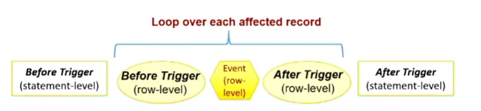
- Two trigger times
- Before the event
- After the event
- Two granularities
- Execute for each row
- Execute for each statement
- Three event types
- CREATE TRIGGER <name>
BEFORE|AFTER INSERT|UPDATE|DELETE ON <tablename> ← the event
FOR EACH ROW|FOR EACH STATEMENT ← the granularity
WHEN <condition> ← the condition
BEGIN
… ← the action
For INSERT events:
Rule 1: Do not use :old variable here (it does not exist)
Rule 2: :new variable gives you the new values to be inserted
For DELETE events:
Rule 1: Do not use :new variable (it does not exist)
Rule 2: :old variable gives you the old values to be deleted
For UPDATE events:
Rule 1: :old gives you the old values before the update
Rule 2: :new gives you the new values after the update
For statement-level trigger (FOR EACH STATEMENT):
Rule 1: Statement-level triggers have no access to :old or :new
END;/ ← end the trigger definition
- A single SQL statement may insert, update, or delete many records at the same time
- The granularity of a trigger allows you to specify if the trigger executes for each updated record, or once for the entire statement
- In Oracle, the default is FOR EACH STATEMENT
- In the action or condition, you may want to reference
- The new values of inserted or updated records (:new)
- The old values of deleted or updated records (:old)
- In UPDATER triggers, can specify which column to observe with BEFORE/AFTER UPDATE OF <column_name> ON <table_name>
- Combine multiple events in one trigger with OR, know the current operation
with
CREATE TRIGGER EmpBonus
BEFORE INSERT OR UPDATE ON Employee
FOR EACH ROW BEGIN
IF (inserting) THEN … ENDIF;
IF (updating) THEN … ENDIF;
END;
/ - Order of trigger inserting
- Important: (Transaction is one unit)
Any any moment, if you cancel the transaction “RAISE_APPLICATION_ERROR”
→ The entire transaction is cancelled/rolled back
→ All the changes in a transaction happen, or none at all - Before vs. Update events
- Before Event
- When checking certain conditions that may cause the operation to be
cancelled
- E.g., if the name is null, do not insert
- When modifying values before the operation
- E.g., if the date is null, put the current date
- When checking certain conditions that may cause the operation to be
cancelled
- After Event
- When taking other actions that will not affect the current operations
- The insert in table X will cause an update in table Y
- When taking other actions that will not affect the current operations
- Before Event
- Row-level vs. statement-level triggers
- Row-level triggers
- Check individual values and can update them
- Have access to :new and :old vectors/tuples
- Statement-level triggers
- Do not have access to :new or :old vectors (only for row-level)
- Execute once for the entire statement regardless how many records are affected
- Used for verification before or after the statement
- Row-level triggers
- Some other operations
- DROP TRIGGER <trigger_name>;
- SHOW ERRORS; → displays the compilation errors
- Check auxiliary tables (DMBS creates these for us) user_triggers and user_trigger_cols for user-defined triggers
- In a row-level trigger, you cannot have the body refer to the table specified in the event as it would see inconsistent data
- Constraints vs. Triggers
- Constraints are useful for database consistency
- Use IC when sufficient
- More opportunity for optimization
- Not restricted to insert/delete/update
- Triggers are flexible and more powerful
- Alerters
- Event logging for auditing
- Security enforcement
- Analysis of table accesses (statistics)
- Workflow and business logic
- But can be hard to understand … - Several triggers (Arbitrary order unpredictable !?) - Chain triggers (When to stop ?) - Recursive triggers (Termination?)
- Constraints are useful for database consistency
- JDBC — Java Database Connectivity API
- Configure system → Connect → Query → Process results → Close
- JDBC requires you to write SQL queries directly in your Java code
- Configure system → Connect → Query → Process results → Close
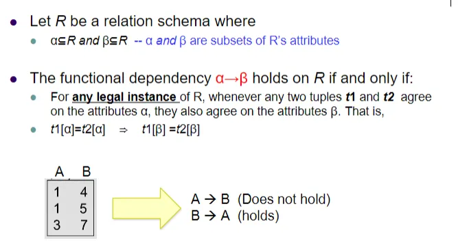
- Functional Dependencies and Normalization
- Functional Dependencies (FDs) - Suppose we have the FD: sNumber → address - Meaning: A student number determines their address - Or: For any two rows in the Student relation with the same sNumber, their addresses must be the same - Require that the value for a certain set of attributes determines uniquely the value for another set of attributes - A functional dependency is a generalization of the notion of a key - Basic form of a FD - A1, A2,…, An → B1, B2,…, Bm - The value on the LHS uniquely determine the values in the RHS attributes - Does not mean that LHS values compute the RHS values - Any key (primary or candidate) or superkey of a relation R functionally determines all attributes of R
- K is a superkey for relational schema R if and only if
- K → R — K determines all attributes of R
- K is a candidate key for R if and only if
- K → R, and
- No a ⊂ K, a → R
- Keys imply FDs, and FDs imply keys
- Properties — Consider sets of attributes A, B, C, Z
- Reflexive (trivial)
- A → B is trivial if B ⊆ A
- Transitive
- If A → B, and B → C, then A → C
- Augmentation
- If A → B, then AZ → BZ
- Union
- If A → B, A → C, then A → BC
- Decomposition - If A → BC, then A → B, A → C
- Reflexive (trivial)
- Closure of a Set of Functional Dependencies
- Given a set F of FDs, there are other FDs that can be inferred based on F
- Closure set F → F+
- The set of all FDs that can be inferred from F
- We denote the closure of F by F+
- F+ is a superset of F
- Computing the closure F+ of a set of FDs can be expensive, but easy
- Recursive apply the transitive property
- Algorithm for computing attribute closures
- Let X = {A1, A2,…, An}+
- If there exists a FD: B1, B2,.., Bm → C, such that every Bi ε X, then X = X U C
- Repeat step 2 until no more attributes can be added
- What are the possible keys for R
- Compute the closure of each attribute X, i.e., X+
- X+ contains all attributes, then X is a key
- Lossy & lossless relation decomposition
- Assume R is divided into R1 and R2
- Lossless decomposition
- R1 natural join R2 should create exactly R
- Lossy decomposition
- R1 natural join R2 adds more records (or deletes records) from R
- The common columns must be candidate key in one of the two relations to ensure lossless decomposition
- Normalization
- A set of rules to systematically achieve a good design
- If these rules are followed, then the DB design is guaranteed to avoid
several problems
- Inconsistent data
- Anomalies: insert, delete, and update
- Redundancy: which wastes storage, and often slows down query processing
- If relation R is not in good form, decompose R
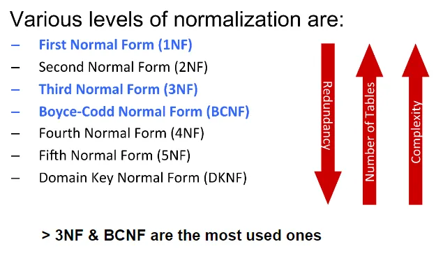
- First normal form (1NF)
- Attribute domain is atomic if its elements are considered to be indivisible units (primitive attributes)
- Examples of non-atomic domains are multi-valued and composite attributes
- A relational schema R is in first normal form (1NF) if the domains of all attributes of R are atomic
- We assume all relations are in 1NF
- A table is considered to be in 1NF if all the fields contain only scalar values
- Boyce-Codd normal form (BCNF)
- A relation schema R is in BCNF with respect to a set of F of functional
dependencies if for all FDs in F+ of the form a → b where a ⊆ R and b ⊆ R,
then at least one of the following holds
- a → b is trivial (i.e., b ⊆ a)
- a is a superkey for R
- If R is not in BCNF because of non-trivial dependency a → b, then decompose
R
- R1 = (a U b) — a is key in R1
- R2 = (R - (b - a)) — R2.a is FK to R1.a
- This decomposition is lossless because R1 and R2 can be joined on a, and a is unique in R1
- Multi-step decomposition
- Is R in BCNF → R1, R2 → are R1 and R2 in BCNF → …
- Drawbacks
- Dependency preservation
- After the decomposition, all FDs in F+ should be preserved, but BCNF does not guarantee dependency preservation
- A decomposition that is both dependency preserving and BCNF may not exist → study a weaker normal form called 3NF
- Dependency preservation
- Dependency preservation test
- R is decomposed into R1 and R2
- Closure of FDs in R is F+
- FDs in R1 and R2 are F(R1) and F(R2) (local dependencies) respectively
- Dependencies are preserved if F+ = (F(R1) U F(R2))+
- A relation schema R is in BCNF with respect to a set of F of functional
dependencies if for all FDs in F+ of the form a → b where a ⊆ R and b ⊆ R,
then at least one of the following holds
- Third normal form (3NF)
- Allows some redundancy but all FDs are preserved
- There is always a lossless, dependency-preserving decomposition in 3NF
- Relation R is in 3NF if, for every FD a → b where a ⊆ R and b ⊆ R, at least
one of the following holds
- a → b is trivial (i.e., b ⊆ a)
- a is a superkey for R
- Each attribute in b - a is part of a candidate key (prime attribute)
- In other words, LHS is superkey or RHS consists of prime attributes
- Canonical cover of FDs
- The smallest set of FDs that produce the same F+
- Canonical cover of F is the minimal subset of FDs (G), where G+ = F+
- Algorithm for minimal cover
- Decompose FD into one attribute on RHS
- Minimize left side of each FD
- Check each attribute on LHS to see if deleted while still preserving the equivalence to F+
- Delete redundant FDs
- Note: several minimal covers may exist
- Theorem: Use minimum cover of FD+ in decomposition guarantees that the decomposition is lossless and dependency preserving when decomposing