Assessment Prep

With a LOT of help from Gemini (hehe). Also, Welch Labs YouTube channel is a goldmine.

Machine learning

Supervised vs unsupervised learning

• Supervised Learning: Learning from data that is labeled. You have a set of input-output pairs and the goal is to learn a function that can map new inputs to their correct outputs ().

  • Analogy: Learning with an answer key.
  • Examples:
    • Classification: The output is a category (e.g., “cat,” “dog,” “spam,” “not spam”).
    • Regression: The output is a continuous value (e.g., $250,000, 1.5, 30.2).

• Unsupervised Learning: Learning from data that is unlabeled. You only have the inputs , and the goal is to discover hidden patterns or structure in the data.

  • Analogy: Learning by observation and finding patterns.
  • Examples:
    • Clustering (e.g., K-Means): Grouping similar data points together.
    • Dimensionality Reduction (e.g., PCA): Compressing the data by finding its most important features.

Loss functions

A loss function (or cost function) measures how “wrong” a model’s prediction is compared to the true label. The entire goal of training is to adjust the model’s weights to minimize the value of this function.

MSE (Mean Squared Error)

• Formula:
• What it is: The average of the squared differences between the true and predicted values.
• When to use: This is the default loss function for regression tasks.
• Intuition: It punishes large errors much more than small errors (because the error is squared). Being off by 4 is worse than being off by 1. This makes it sensitive to outliers.

Cross-entropy

• What it is: Measures the “distance” between two probability distributions: the true labels (e.g., [0, 1, 0]) and the predicted probabilities (e.g., [0.1, 0.8, 0.1]).
• When to use: This is the default loss function for classification tasks.
• Intuition: It penalizes the model heavily for being confidently wrong. If the true class is 1 and the model predicts 0.001, the loss is huge (). It forces the model to assign a high probability to the correct class.

Hinge loss

• Formula: (where is -1 or 1).
• When to use: Primarily for Support Vector Machines (SVMs).
• Intuition: It doesn’t care about predictions that are “correct enough.” If the true label is 1 and the model predicts 1.5, the loss is 0. It only applies a penalty if the prediction is not “confidently correct” (i.e., not on the right side of the “margin”).

Cross-validation

• The Problem: How do you get a reliable estimate of your model’s performance on unseen data? A simple train/test split might be “lucky” or “unlucky.”
• The Solution: K-Fold Cross-Validation
  1. Divide your training dataset into equal-sized “folds” (e.g., ).
  2. Train separate models.
  3. Model 1: Train on folds 2, 3, 4, 5. Validate on fold 1.
  4. Model 2: Train on folds 1, 3, 4, 5. Validate on fold 2.
  5. …and so on.
• The Result: You get validation scores. The average of these scores is a much more robust estimate of how your model will perform.

Hyperparameter tuning

• What it is: The process of finding the optimal “settings” for a model that are not learned during training.
• Parameters vs. Hyperparameters:
  • Parameters are learned (e.g., the weights and biases in a neural network).
  • Hyperparameters are set by you (e.g., the learning rate, the number of layers, the choice of optimizer like Adam vs. SGD).
• Common Methods:
  • Grid Search: Tries every possible combination from a list you provide (e.g., learning_rate=[0.1, 0.01], layers=[2, 4, 8]). Very slow.
  • Random Search: Tries random combinations. Often more efficient than grid search.

Overfitting and underfitting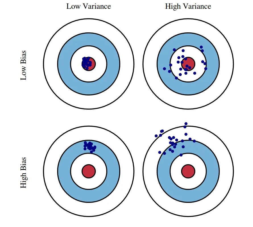

• Underfitting (High Bias):

  • Symptom: The model performs poorly on the training data (and also on the test data).
  • Cause: The model is too simple to capture the underlying pattern in the data (e.g., using a linear model for a complex, non-linear problem).
  • How to Fix: Use a more complex model (e.g., add more layers, more neurons).

• Overfitting (High Variance):

  • Symptom: The model performs great on the training data but poorly on the test data.
  • Cause: The model is too complex and has “memorized” the noise and specific examples in the training set instead of learning the general pattern.
  • How to Fix:
    1. Get more data: The best defense.
    2. Regularization: Add a penalty for complexity (e.g., L1, L2, Dropout).
    3. Early Stopping: Stop training when the validation loss starts to increase.
    4. Data Augmentation: Artificially create more training data (e.g., flip, rotate, or crop images).

Deep learning

Backpropagation

• What it is: The algorithm used to train neural networks. It’s how the network learns by “assigning blame” for its errors to every weight.
• How it Works (Intuitively):
  1. Forward Pass: Make a prediction and calculate the loss (the error).
  2. Backward Pass: This is just the chain rule from calculus.
  3. You start at the end: find the derivative (gradient) of the loss with respect to the last layer’s weights. This tells you “how much does the loss change if I ‘nudge’ this weight?”
  4. You “propagate” this gradient backward, layer by layer, calculating the gradient for all weights, all the way back to the first layer.
  5. Weight Update: The optimizer (like SGD) uses these gradients to update every single weight in the network, “nudging” them in the direction that minimizes the loss.

MLP (Multi-Layer Perceptron)

• What it is: The most basic “classic” neural network architecture.
• Structure:
  1. An Input Layer (holds your raw data).
  2. One or more Hidden Layers.
  3. An Output Layer (makes the final prediction).
• Each hidden layer is “fully connected” (or “dense”), meaning every neuron in that layer is connected to every neuron in the previous layer.
• Each layer’s operation is a linear step (matrix multiplication ) followed by a non-linear activation function (like ReLU). This non-linearity is essential; without it, a 100-layer network would just be a single, simple linear model.

CNN (Convolutional Neural Network)

Filters

A filter (or kernel) is the fundamental component of a convolutional layer. It’s a small, learnable matrix of weights (e.g., or ).

• Intuition: Think of it as a feature detector. Each filter learns to “look for” one specific, simple pattern in the image.
• Process: In the first layer, filters learn to detect low-level features like vertical edges, horizontal edges, specific colors, or simple textures.
• Visualization: If you visualize the weights of a trained filter, it often looks like the very pattern it’s trying to find. Techniques like feature visualization can generate images that “excite” a specific filter, showing us what pattern it has learned to recognize.

Convolutional layers

A convolutional layer’s job is to apply its set of filters to an input volume (like the initial image or the feature map from a previous layer).

• Operation: The layer “slides” each filter across the entire input, one step at a time. At every single position, it computes the dot product between the filter’s weights and the small patch of the image it’s currently on.
• Output (Feature Map): This sliding dot-product operation produces a 2D output called a feature map or activation map.
• Intuition: This activation map is a 2D grid that shows where the filter’s specific feature (e.g., “vertical edge”) was found in the input. A high value means a strong match for the feature at that location.
• Stacking: A single convolutional layer learns many filters (e.g., 64 or 128) in parallel. It applies all of them to the input, producing a stack of 64 or 128 different feature maps. This 3D tensor is then passed as the input to the next layer.

Pooling

A pooling layer is a non-learnable layer that performs downsampling. Its goal is to progressively reduce the spatial size (width and height) of the feature maps.

• How (Max Pooling): The most common type is max pooling. It works by sliding a small window (e.g., ) across the feature map. At each position, it outputs only the maximum activation value from that window, discarding the rest.
• Two Main Purposes:
  1. Computational Efficiency: It drastically reduces the number of parameters and the amount of computation in the network.
  2. Local Invariance: It makes the feature detection more robust. By taking the max, the network only cares that a feature was present in a small region, not its exact pixel location. This helps the model recognize an object even if it’s slightly shifted or scaled.

AlexNet

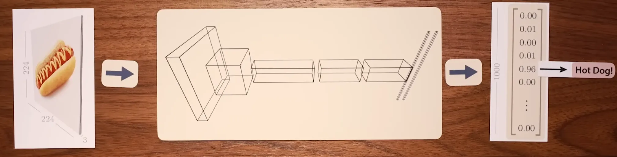
• Classifies image inputs into 1000 different classes
• Input is 224 x 224 x 3 image processed as a tensor
• Output is probabilities across 1000 classes
• CNN block
  • First developed in 1980s to recognize handwritten digits
  • Can be understood as a special case of the transformer block
• Kernel is a much smaller tensor of learned weights used to slide across the input image and compute the dot product at each position to produce a feature map/activation map. 1 kernel produces 1 activation map.
  • Can think of dot product as similarity score
• Intuition: the activation maps are images themselves and can be used to visualize which part of the input image matches the kernel (which is an image as well) well
• These activation maps are then stacked into a tensor and fed into the next CNN block. This process repeats.
• Intuition: as we move deeper into AlexNet, strong activations map to higher-level features (e.g., wheels, eyes) instead of low-level features (e.g., edges, colors)
  • Example: By the 5th layer, there are activation maps that respond very strongly to faces
• Feature visualization
  • Technique to generate synthetic images that maximize the activation of specific kernels
  • Visualize what each kernel is looking for in the input image
  • Start with random noise image and iteratively modify it using gradient ascent to maximize the activation of a specific kernel in a specific layer
  • After many iterations, the resulting image reveals the patterns that the kernel is sensitive to
  • Helps understand what features the network has learned to recognize at different layers

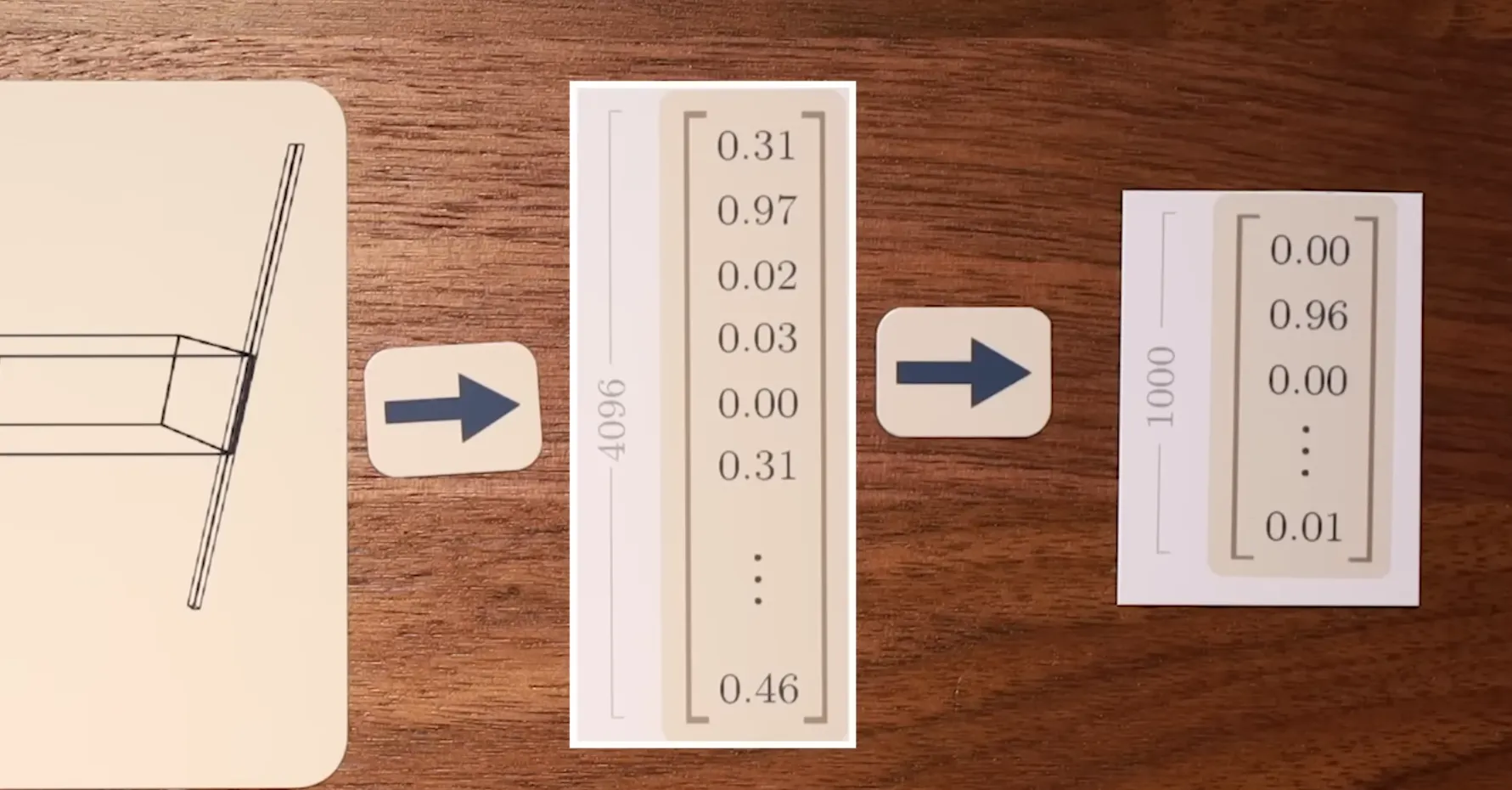
• The second-to-last output is a 4096-dimensional vector which goes through a final fully-connected layer to produce the 1000 class probabilities
  • Can think of this as a point in a 4096-dimensional space, also called latent/embedding space
  • When measured the distance between these points for different images, images of similar classes are closer together in this space

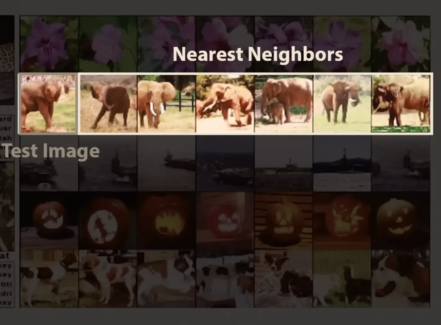
• Nearest neighbors (vector distance) in this space to this feature vector shows semantically similar images
• Not only distance but also direction matters
  • Example: vector arithmetic in this space shows that vec("king") - vec("queen") = vec("man") - vec("woman")
  • Application: age/gender shift in face
    • vec("Alice") - vec("young Alice") + vec("young Eve") = vec("Eve")
• Latent space walking
  • Interpolating between two points in this space produces smooth transformations between the two images when decoded back to image space
  • Application: style transfer, image morphing

RNN (Recurrent Neural Network)

• Purpose: Designed for sequence data where order matters (e.g., text, time series).
• Core Idea: A loop. The network has a “hidden state” (its memory).
  1. It processes the first token (e.g., “hello”) and produces an output and a new hidden state.
  2. To process the next token (“world”), it takes two inputs: the new token and the hidden state from the previous step.
• The Problem: Vanishing Gradients. When backpropagating through many time steps, the “blame” signal can shrink to zero, making it impossible for the model to learn long-term dependencies (e.g., remembering a word from 50 tokens ago).

LSTM (Long Short-Term Memory)

• Purpose: A special type of RNN cell designed to solve the vanishing gradient problem.
• Core Idea: It maintains a separate Cell State (), which acts as a “long-term memory” conveyor belt. It uses three “gates” (small, internal networks) to control this memory:
  1. Forget Gate: Decides what old information to throw away from the cell state.
  2. Input Gate: Decides what new information to write to the cell state.
  3. Output Gate: Decides what part of the cell state to read and use for its output/hidden state.
• This structure allows important information to flow unchanged for long distances, enabling the model to learn long-term dependencies.

GRU (Gated Recurrent Unit)

• Purpose: A simplified, more computationally efficient version of an LSTM.
• Core Idea: It combines the “forget” and “input” gates into a single Update Gate. It also merges the cell state and hidden state.
• Result: It has fewer parameters than an LSTM and trains faster. It often performs just as well and is a very common choice.

Transformer

Consists of an attention block feeding into a MLP block.

ChatGPT

• Generates text one token at a time given an input prompt
• The input text is split into tokens. Each token is assigned a unique integer ID based on a predefined vocabulary. These IDs are used to index into an embedding matrix (usually of fixed size) to convert tokens into dense vectors. This sequence of vectors (matrix) is the input to the model.
  • Example: ["Hello", "world", "!"] -(tokenizer)-> [123, 456, 789] -(embedding matrix of shape [vocab_size, embedding_dim] (100,000 tokens x 768 dimensions))-> [[0.25, -0.13, ..., 0.04], [0.02, 0.98, ..., -0.11], [-0.33, 0.07, ..., 0.56]]
  • Embeddings are treated as a layer in the neural network and are learned during training.
• The output is a probability distribution over the vocabulary for the next token
• Various output sampling strategies select the next token based on this distribution during inference. While in training, the most probable token is used to compute the loss.
• Output tokens are converted back to text using the tokenizer’s reverse mapping from token IDs to words or subwords and appended to the input.
• Repeat the process until the desired length or an end-of-sequence token is generated.
• Loss function is cross-entropy loss between predicted token probabilities and actual next tokens in the training data.

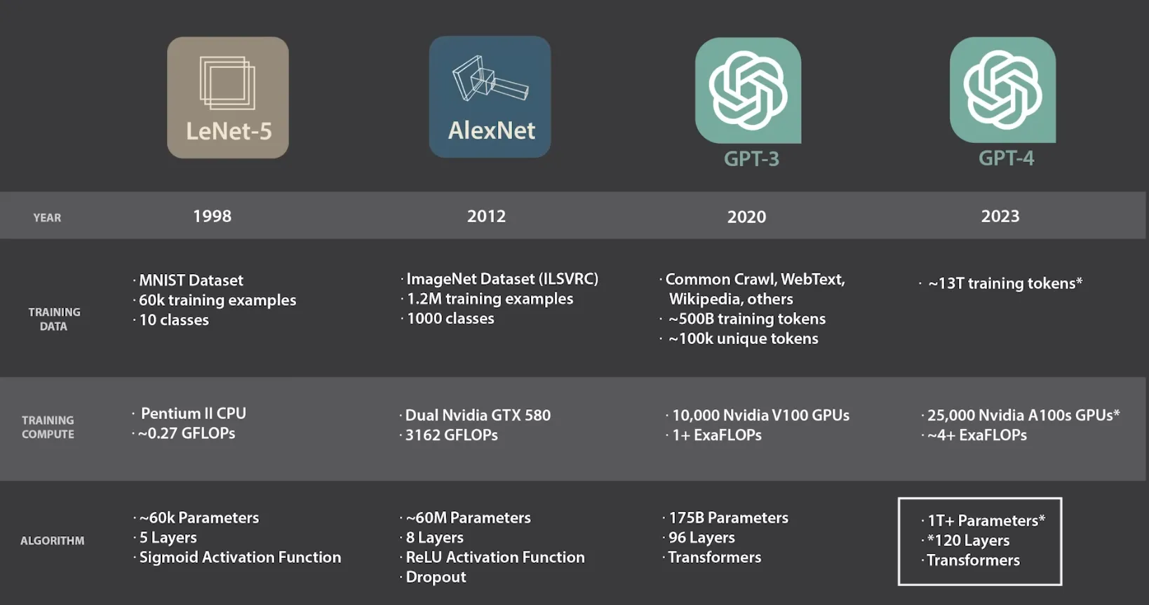
• Scale of data and compute enables higher model capacity and better generalization

Neural scaling laws

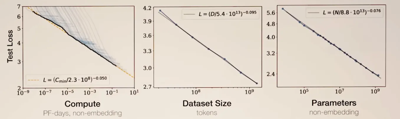
NVIDIA Tesla V100 GPU can deliver 28 TeraFLOP/s of FP16 compute. 33 of them make up 1 PetaFLOPs.

Manifold hypothesis: Why model performance is so simply predicted by compute and data following a power law? One possible explanation is that deep learning models use data to resolve a high-dimensional data manifold. Can think of image, text, and data as points on this high-dimensional manifold. Essentially models turn high-dimensional input spaces to lower-dimensional manifolds where the position of data on the manifold is meaningful.

Natural data (images, language, etc.) live on a low-dimensional manifold embedded in a high-dimensional ambient space (e.g., pixels, tokens).

Attention

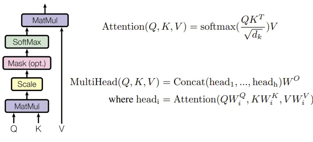
Q, K, and V are all learnable parameters (matrices) that transform the input vectors into different “views” for computing attention.

k is hyperparameter shared between Q, K, V

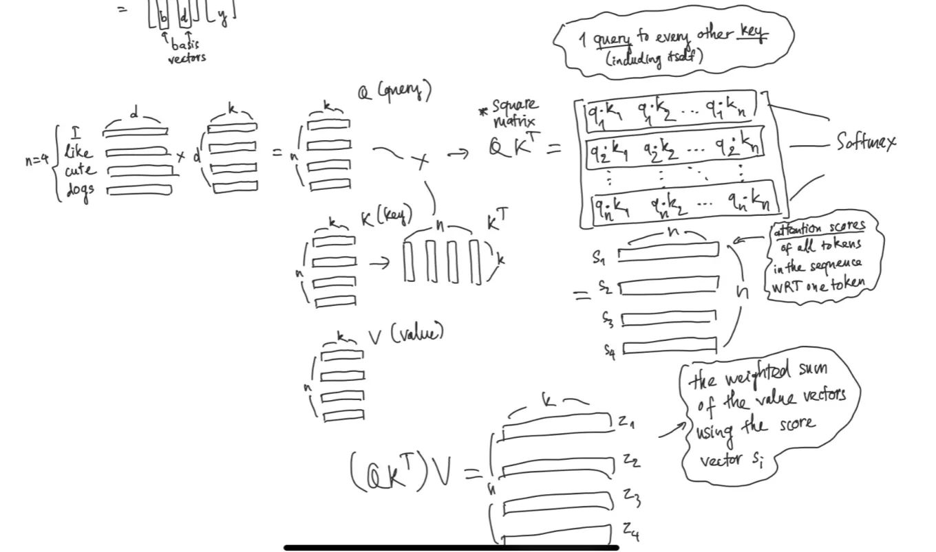
• Purpose: The core mechanism of the Transformer. It solves the sequence problem without recurrence (loops), allowing for massive parallelization.
• Core Idea: For every token in a sequence, it looks at every other token and calculates an “attention score” that determines how “important” each other token is for understanding the current one.
• Query, Key, Value (QKV):
  1. Each token creates three vectors: a Query (“What am I looking for?”), a Key (“What information do I have?”), and a Value (“What I will provide”).
  2. To get the score for one token, its Query is dot-producted with every other token’s Key (including itself).
  3. These scores are run through a softmax to create weights (summing to 1).
  4. The final output for that token is the weighted sum of all tokens’ Value vectors.
• This allows the model to directly connect “it” to “animal” in a long sentence, no matter how far apart they are.

Encoder-decoder architecture

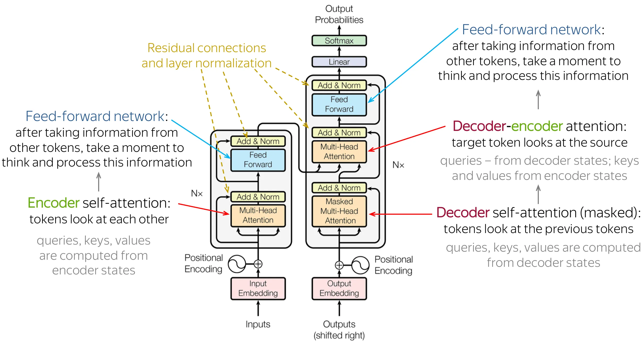
• Purpose: The original Transformer architecture, built for sequence-to-sequence tasks (like machine translation).
• The Encoder (Left Stack):
  • Its job is to “read” and “understand” the input sentence.
  • It’s a stack of blocks containing Self-Attention (so input words can look at each other) and an MLP.
  • It outputs a set of contextualized feature vectors for the input.
• The Decoder (Right Stack):
  • Its job is to “generate” the output sentence, token by token.
  • It has two attention mechanisms:
    1. Masked Self-Attention: Looks at the output tokens it has already generated (it’s “masked” so it can’t “cheat” and see future tokens).
    2. Cross-Attention: Its Queries come from the decoder, but its Keys and Values come from the Encoder’s output. This is how the decoder “pays attention” to the input sentence to decide what to translate next.

BatchNorm, LayerNorm, weight initialization

• The Problem: Training deep networks is unstable. The distribution of inputs to each layer (the “activations”) changes during training, a problem called “internal covariate shift.”
• Weight Initialization:
  • What: How we set the initial random weights.
  • Why: If weights are too big, activations explode; if too small, they vanish.
  • Solution: Smart initialization schemes like Xavier/Glorot (for tanh) or He (for ReLU) set the initial variance of weights based on the layer size to keep the signal flowing.
• BatchNorm (Batch Normalization):
  • What: A layer that re-normalizes activations during training.
  • How: It normalizes across the batch, forcing the activations to have a mean of 0 and stddev of 1.
  • Effect: Drastically stabilizes training, allows for much higher learning rates, and speeds up convergence.
• LayerNorm (Layer Normalization):
  • What: An alternative, used in Transformers.
  • How: It normalizes across the features/dimensions for a single training example, instead of across the batch.
  • Effect: It’s independent of batch size, which is critical for NLP where sequences have variable lengths.

Optimizers (Adam, SGD, RMSProp)

• Purpose: The algorithm that uses the gradient (from backpropagation) to update the model weights.
• SGD (Stochastic Gradient Descent):
  • How: The simplest. weight = weight - learning_rate * gradient.
  • Problem: Can be slow or get stuck in local minima.
  • SGD + Momentum: Adds a “velocity” term. The update is like a heavy ball rolling downhill, building momentum to push past small bumps.
• RMSProp (Root Mean Square Propagation):
  • How: An adaptive optimizer. It maintains a moving average of the squared gradients.
  • Intuition: It divides the learning rate by the square root of this average. This reduces the update for “loud” gradients and increases it for “quiet” ones, adapting the learning rate per-parameter.
• Adam (Adaptive Moment Estimation):
  • How: The default choice for most problems. It’s essentially RMSProp + Momentum.
  • Intuition: It keeps a moving average of both the gradient (like momentum) and its squared value (like RMSProp).

Transfer learning and fine-tuning

• Core Idea: Don’t train a massive model from scratch. Use a model that has already been trained on a giant, general dataset.
• The Process:
  1. Pre-training: A huge model (e.g., BERT, AlexNet) is trained on a massive dataset (e.g., all of Wikipedia, ImageNet). This model learns general features about language or images.
  2. Fine-tuning:
     • Take this pre-trained model.
     • Chop off its final output layer.
     • Add a new output layer for your specific task (e.g., a 2-class layer for sentiment analysis).
     • Train this modified model on your small, specific dataset using a very low learning rate.
• Why: It’s dramatically faster, cheaper, and more accurate than training from scratch, especially when you have limited data.

NLP

Tokenization

Byte-pair encoding (BPE)

• What: A common subword tokenization algorithm.
• How it Works:
  1. Starts with a vocabulary of all individual characters (bytes).
  2. Iteratively finds the most frequent pair of adjacent tokens in the corpus.
  3. Merges this pair into a new, single token and adds it to the vocabulary.
  4. Repeats this times (e.g., for a vocab size of 30,000).
• Result: Common words (“the”) become single tokens. Uncommon words (“tokenization”) become ["token", "ization"]. Can handle any word, so there are no unknown tokens.

WordPiece

• What: The subword algorithm used by BERT.
• How it Works: Very similar to BPE, but it merges the pair that maximizes the likelihood of the training data, rather than just the most frequent pair. It’s a slightly different statistical-based merge criterion, but the intuition is the same.

SentencePiece

• What: A tokenizer (and library) used by models like Llama.
• Key Feature: It treats spaces as a normal character (e.g., by replacing ” ” with ” ”). This means it can tokenize directly from raw text without any special pre-processing to split on spaces, making it a “cleaner” end-to-end system.

Stemming

• What: A crude, rule-based process for chopping off word endings to get the “stem.”
• Example: “running,” “runs” -> “run.” “computation” -> “comput.”
• Problem: It’s very aggressive and often creates non-words (“comput”).

Lemmatization

• What: A “smarter,” dictionary-based process to find the root “lemma” of a word.
• Example: “running,” “runs,” “ran” -> “run,” “run,” “run.” (It knows “ran” is the past tense of “run”).
• Tradeoff: More accurate than stemming, but much slower. (Modern subword tokenizers largely replace both).

Traditional representations

Bag-of-words

• What: The simplest way to represent a document as a vector.
• How:
  1. Define a vocabulary of all possible words (e.g., 50,000 words).
  2. Represent a document as a 50,000-dimension vector where each index is the count of how many times that word appeared.
• Problem: Loses all word order and context. “The dog bit the man” and “The man bit the dog” look very similar.

TF-IDF

• What: An upgrade to Bag-of-Words. It represents a document as a vector of importance scores, not just counts.
• How: The score for a word is a product of two terms:
  1. TF (Term Frequency): How often the word appears in this document. (Same as BoW).
  2. IDF (Inverse Document Frequency):
• Intuition: The highest scores go to words that are frequent in this document but rare in all other documents. It filters out common, “stop” words like “the” and “a” which have a low IDF score.

Word embeddings

Word2Vec

• What: An algorithm to learn dense word embeddings (vectors).
• How it Works (Two main ways):
  1. Skip-Gram: You give the model a word (e.g., “king”) and it tries to predict the surrounding context words (e.g., “a,” “is,” “on,” “his,” “throne”).
  2. CBOW (Continuous Bag-of-Words): You give the model the context words (e.g., [“a,” “is,” “on,” “his,” “throne”]) and it tries to predict the center word (“king”).
• Key Idea: The trained model is thrown away. The weights of its internal hidden layer are kept as the word embeddings.
• Result: The vectors capture semantic meaning (e.g., ).

GloVe (Global Vectors)

• What: An alternative embedding-learning algorithm.
• How it Works: Instead of a “fake” prediction task, it directly optimizes vectors to explain global statistics.
  1. It first builds a giant co-occurrence matrix (how often does “king” appear near “queen”?).
  2. It then uses matrix factorization to directly learn vectors that best explain the ratios of these co-occurrence probabilities.
• Difference: Word2Vec is “local” (uses a sliding window). GloVe is “global” (uses corpus-wide statistics).

FastText

• What: An extension of Word2Vec (Skip-Gram).
• Key Difference: It learns vectors for character n-grams (e.g., 3-grams for “where” are whe, her, ere).
• The final vector for a word is the sum of its n-gram vectors.
• Main Benefit: It can generate vectors for out-of-vocabulary (OOV) words. If it sees a typo like “toknization,” it can still build a reasonable vector from its parts (e.g., tok, okn, kni…), whereas Word2Vec would just map it to an “unknown” token.

Tasks

Text classification

• What: Assigning a single categorical label to a piece of text.
• Example:
  • Topic Classification: “sports,” “politics,” “tech.”
  • Spam Detection: “spam,” “not spam.”
  • Sentiment Analysis: (See below).

Sentiment analysis

• What: A specific type of text classification.
• Task: Assigning a label that reflects the “opinion” or “feeling” of the text.
• Example:
  • Labels: “positive,” “negative,” “neutral.”
  • Use Case: Analyzing movie reviews, product feedback, or social media posts.

Machine translation

• What: A sequence-to-sequence task.
• Task: Taking a sequence (sentence) in one language as input and generating a sequence (the same sentence) in another language as output.
• Classic Architecture: The Encoder-Decoder Transformer.

Question answering

• What: Answering a question based on a given context paragraph.
• Task (Extractive QA): The model doesn’t “generate” an answer; it predicts the span of text in the context that contains the answer.
• Input: A (context, question) pair.
• Output: A (start_index, end_index) pair.

Retrieval-augmented generation (RAG)

• The Problem: Large Language Models (LLMs) “hallucinate” (make up facts) and their knowledge is “frozen” at the time they were trained.
• The Solution (RAG):
  1. Retrieve: When a user asks a question, first use that question to search a database (a vector database) of up-to-date or private documents.
  2. Augment: Take the most relevant documents (the “context”) and “stuff” them into the LLM’s prompt along with the user’s original question.
  3. Generate: Ask the LLM to answer the question using only the provided context.
• Result: This dramatically reduces hallucinations and allows the LLM to answer questions about new or private information.