Transformer architecture

Training

Training involves feeding large datasets of text into the model. A contiguous text block of size context_len is sampled from from the train set, and the model is trained to predict the next token at each position in the text block i.e. a block of 9 characters has 8 examples.

This is not only done for efficiency, but also to help the model learn to get used to making predictions on inputs of variable length from 0 up to context_len during inference.

Embedding

The input text is first tokenized into discrete tokens (subwords, words, or characters) using a tokenizer. Each token is then mapped to a continuous, high-dimensional vector using an embedding table. The embedding table is a learned parameter of size (V, C), where V (vocab size) is the number of unique tokens in the tokenizer and C (channels) is the embedding dimension.

Intuition: If the dot product between two token embeddings is high, they are more related in meaning.

Intuition: Similar tokens (e.g., “cat” and “dog”) land on same neighborhoods in the embedding space, allowing the model to generalize better.

Positional embedding

Other than vocab-based embedding, position embedding is also added to the token embedding to give the model information about the order of the tokens. The embedding table is the usual (T, C) dimension, where T (time step) is the maximum context length and C (channels) is the embedding dimension.

Attention

These sequence of embeddings are then passed through an attention block. Attention is a parallel operation that gives individual token embeddings the chance to interact with each other and refine the meanings they encode based on the surrounding context.

For example, the embedding for the word “bank” in the sentence “I went to the bank” versus the sentence “The river bank was flooded” should be different.

Intution: Attention moves the embedding vector around in the embedding space based on the context so that the final embedding is more accurate and contextual. A well-trained attention block should move the embedding of “bank” closer to “money” in the first sentence and closer to “river” in the second sentence as a function of the context.

A big part of attention’s success is not because of some specific behavior it enables, rather it’s the massively parallel nature of the operation. And as we have seen from the bitter lesson of deep learning, more parallelism = more scalability = better performance > hard-coded systems.

Mathematical trick in self-attention

In an older representation called bag-of-words, the context is a mixture of all the embeddings of the words in the input, without any positional information. Mean of the embeddings is one example. The embedding of the context is the mean of all embeddings along the embedding dimensions. We calculate this by keeping a running sum and dividing at each time step to get. Instead of running a for loop, it can be calculated in parallel using matrix multiplication as weighted aggregation.

b = torch.randint(0, 10, (3, 2)).float()
# tensor([[2., 9.],
#         [2., 5.],
#         [8., 1.]])
result = torch.zeros_like(b)

# instead of
for i in range(b.shape[0]):
    result[i] = b[: i + 1].mean(dim=0)

# do this
a = torch.tril(torch.ones(b.shape[0], b.shape[0]))
# tensor([[1., 0., 0.],
#         [1., 1., 0.],
#         [1., 1., 1.]])
a = a / a.sum(dim=1, keepdim=True)
# tensor([[1.0000, 0.0000, 0.0000],
#         [0.5000, 0.5000, 0.0000],
#         [0.3333, 0.3333, 0.3333]])
result = a @ b

The half-triangular matrix a is used to mask out future information (upper half all zeroes) and weights the past information equally (lower half all ones, normalized). This weight/affinity matrix signifies the importance of different past tokens to the current one being generated. This is important later on when we want to vary them through training.

Finally, using softmax instead of simple normalization is more generalizable to equal-weight and variable-weight cases.

tril = torch.tril(torch.ones(3, 3))
wei = torch.zeros((3, 3))
wei = wei.masked_fill(tril == 0.0, float("-inf"))
# tensor([[0., -inf, -inf],
#         [0., 0., -inf],
#         [0., 0., 0.]])
wei = wei.softmax(dim=1)
# tensor([[1., 0., 0.],
#         [1., 1., 0.],
#         [1., 1., 1.]])

How it works

Each token embedding is transformed into three vectors: query, key, and value using learned linear projections.

The query represents what the token is looking for in the context (a question asked to other tokens). The key represents what the token has to offer to other tokens (an answer to questions from other tokens). The value represents the actual content of the token.

The Q, K, V dimensions are typically smaller than the embedding dimension C to reduce computational cost. In GPT-3, d_embedding is 12,288 and d_query is 128.

Intuition: Linear projection of the embedding vector from the embedding space to a lower-dimension query/key space that attempts to encode some questions or carry some answers. If the dot product of the query and key in this query/key space is high, the key matches the query very well i.e., “answering the query”.

Attention pattern

To measure how well each key answers each query, we take the dot product between all queries and keys to get an attention score matrix of size (T, T).

attn_scores = keys @ queries.T # (T, T)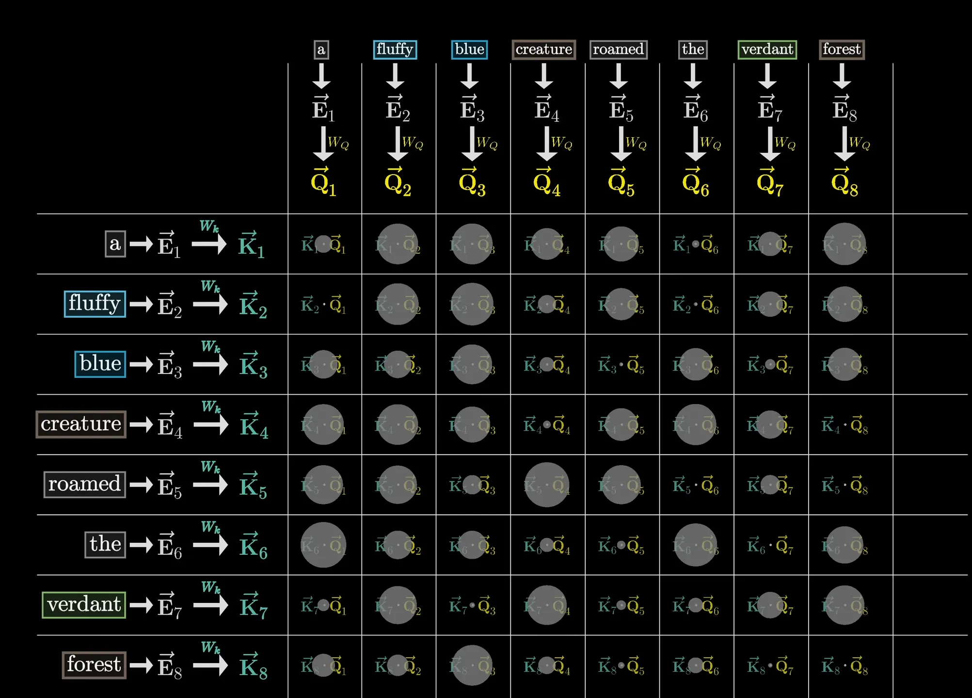

Lingo: if the dot products are high, we say the embeddings of “fluffy” and “blue” attend to the embedding of “creature”.

The meaning of the entries in the attention score matrix is that they are weights/logits for how relevant each token is to updating the meaning of every other token. Softmax comes into play here to convert each column into a probability distribution. And because we’re making an autoregressive language model, keys from the future cannot be used to answer queries from the past, so we mask out the lower triangle of the attention score matrix before softmax. For numerical stability, we also scale the scores by the square root of the query/key dimension (quite similar to Xavier initialization).

Note how attention pattern scales O(T^2) with context length T, which is a big bottleneck for LLMs. There have been many attempts to reduce this cost with sparse attention patterns.

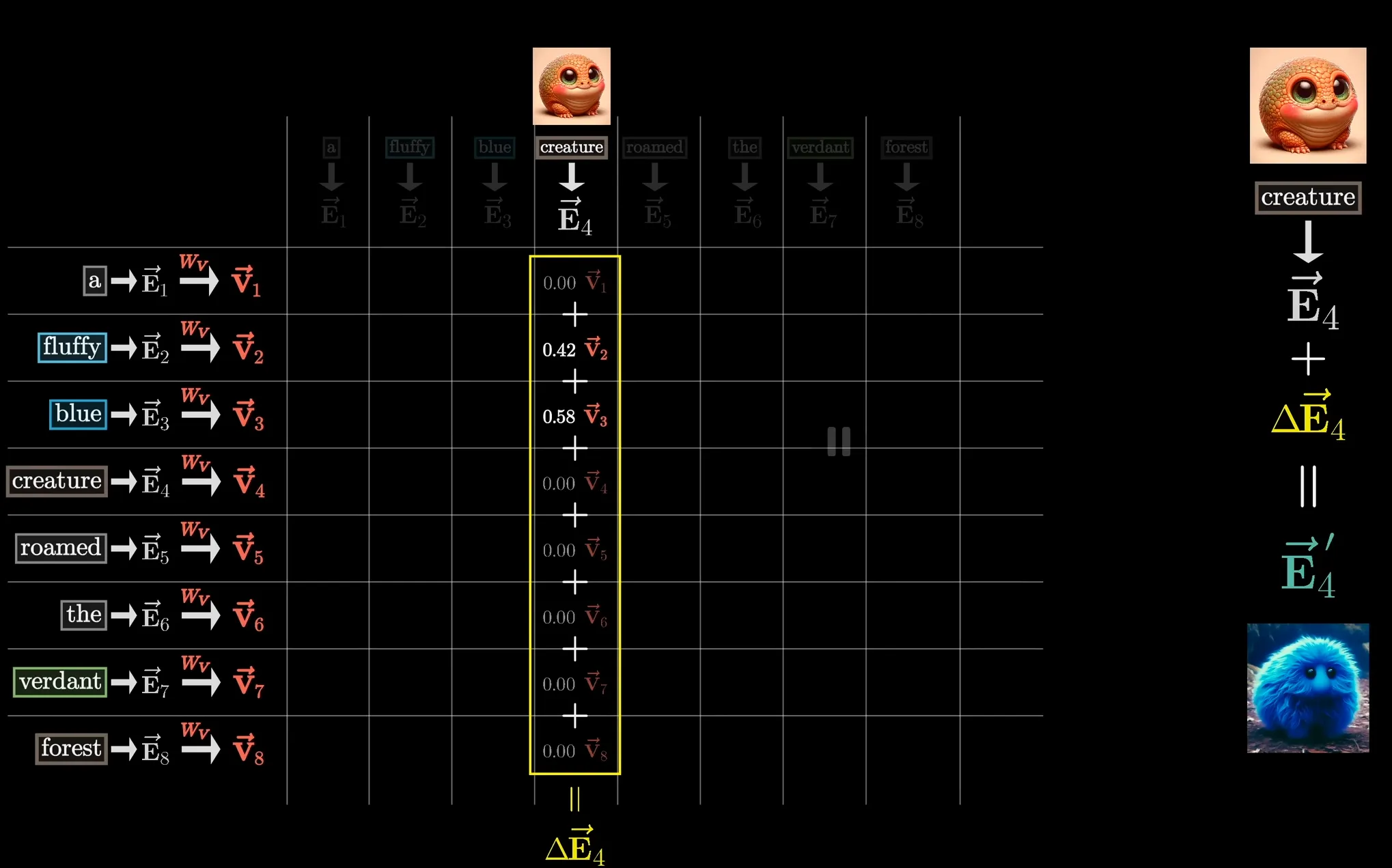
Attention mechanism

Finally, as stated earlier, we want to update the embedding of each token based on the context of its past token. The most straightforward way in the context of single-head attention is to take another weight matrix (the value matrix), matrix multiply it with the original embedding to get the value vector, and add the value vector to the target embedding to get the modified embedding.

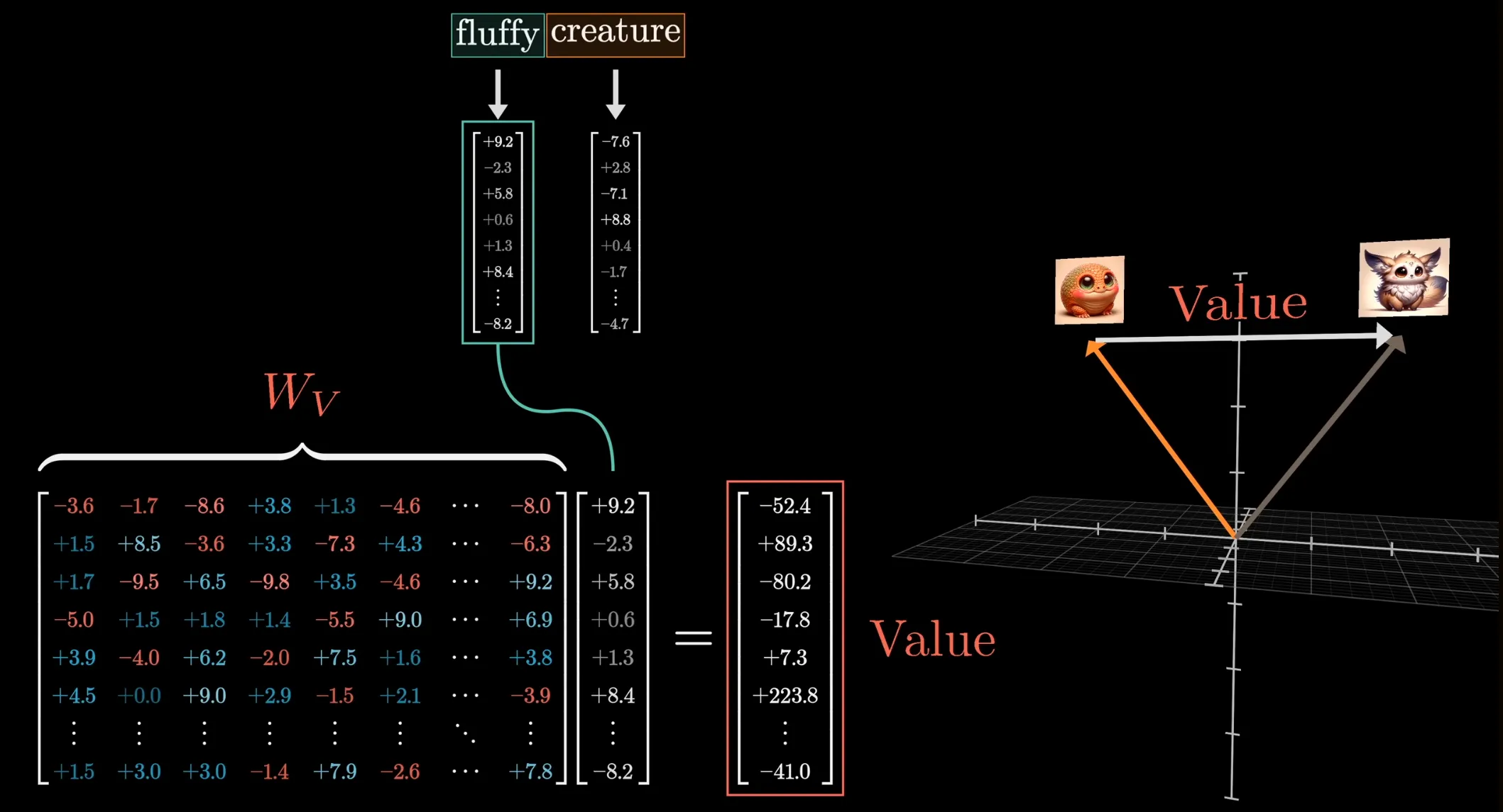
Intuition: If this word is relevant to adjusting the meaning of something else, what exactly should be added to the embedding of that something else in order to reflect this?

Multiple attention heads

A full attention block inside a transfomer layer consists of multiple attention heads, each with its own set of learned linear projections for Q, K, V. For each token, each of the heads proposes a change to the embedding in that position. Then the proposed changes are summed together and added to the original embedding.

In practice though, each head’s output is concatenated together and passed through a final linear projection to get back to the original embedding dimension, which is then added to the original embedding as a residual connection.

PyTorch example

B, T, C = 2, 4, 16
D_head = 8
embeddings = torch.randint(0, 5, (B, T, C)).float()
W_q = torch.randint(0, 5, (C, D_head)).float()
W_k = torch.randint(0, 5, (C, D_head)).float()
W_v = torch.randint(0, 5, (C, D_head)).float()
queries = embeddings @ W_q  # (B, T, D_head)
keys = embeddings @ W_k  # (B, T, D_head)
values = embeddings @ W_v  # (B, T, D_head)

attn_scores = queries @ keys.transpose(-2, -1) / D_head**0.5  # (B, T, D_head) @ (B, D_head, T) -> (B, T, T)
mask = torch.tril(torch.ones(T, T))  # mask out future tokens
attn_scores = attn_scores.masked_fill(mask == 0.0, float("-inf"))
attn_weights = F.softmax(attn_scores, dim=-1)  # (B, T, T)
residuals = attn_weights @ values  # (B, T, T) @ (B, T, D_head) -> (B, T, D_head)
print(embeddings[0])
# tensor([[3., 4., 1., 2., 3., 0., 1., 4., 0., 1., 4., 1., 3., 1., 1., 4.],
#         [0., 1., 0., 3., 4., 3., 1., 4., 1., 3., 4., 4., 1., 2., 4., 3.],
#         [3., 4., 0., 0., 4., 4., 1., 3., 1., 3., 4., 4., 4., 0., 0., 1.],
#         [2., 0., 0., 0., 1., 0., 4., 2., 4., 3., 2., 2., 0., 2., 3., 3.]])
print(attn_weights[0]) # how much each token attends to every other past token
# tensor([[1., 0., 0., 0.],
#         [0., 1., 0., 0.],
#         [0., 1., 0., 0.],
#         [0., 1., 0., 0.]])
print(values[0]) # how much each token has to offer to every other token
# tensor([[23., 60., 44., 55., 67., 81., 52., 67.],
#         [30., 69., 53., 66., 78., 72., 69., 65.],
#         [28., 68., 48., 62., 73., 75., 64., 66.],
#         [25., 39., 49., 58., 49., 48., 45., 52.]])
print(residuals[0]) # how each token's embedding is updated based on the context
# tensor([[23., 60., 44., 55., 67., 81., 52., 67.],
#         [30., 69., 53., 66., 78., 72., 69., 65.],
#         [30., 69., 53., 66., 78., 72., 69., 65.],
#         [30., 69., 53., 66., 78., 72., 69., 65.]])

Karpathy notes

Notes:

• Attention is a communication mechanism. Can be seen as nodes in a directed graph looking at each other and aggregating information with a weighted sum from all nodes that point to them, with data-dependent weights.
• There is no notion of space. Attention simply acts over a set of vectors. This is why we need to positionally encode tokens.
• Each example across batch dimension is of course processed completely independently and never “talk” to each other
• In an “encoder” attention block just delete the mask, allowing all tokens to communicate. This block here is called a “decoder” attention block because it has triangular masking, and is usually used in autoregressive settings, like language modeling.
• “self-attention” just means that the keys and values are produced from the same source as queries. In “cross-attention”, the queries still get produced from x, but the keys and values come from some other, external source (e.g. an encoder module)
• “Scaled” attention additionally divides the weights by . This makes it so when input Q, K are unit variance, weights will be unit variance too and softmax will stay diffuse and not saturate too much.

MLPs

One thought of what might MLPs do in the context of LLMs is that they store facts. An idea floating around interpretability research these days is superposition.

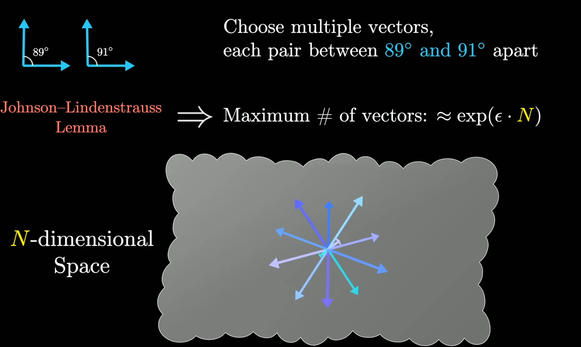
The number of vectors you can cram into a N-dimensional space grows exponentially with N if you allow the vectors to be almost-orthogonal. This is called superposition. By Johnson-Lindenstrauss lemma:

This means that a 12,288-dimensional embedding space (as in GPT-3) can store an enormous amount of almost-orthogonal vectors, each representing a fact/meaning, much more than a 3-dimensional space could. This may also explain why LLMs benefit so much from scaling up the parameter count.

However, as a result, a neuron in the MLP cannot correspond to a single fact, rather a fact is a superposition of many neurons. Sparse autoencoders are one tool for interpretability researchers to try to disentangle these superpositions.

Transformer

Consists of an attention block feeding into a MLP block. This formation repeats for many layers.

GPT-3 matrices

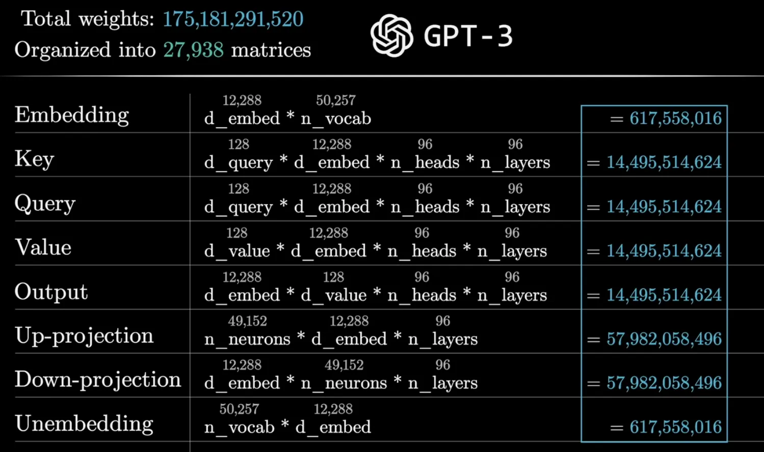
Unembedding

The final step to give the desired output token is unembedding. The first step in this process is to map from the very last embedding vector in the context to the original vocabulary. This is done by matrix multiplying the unembedding matrix of size (V, C) with the final vector of size (C, 1) to get a logits vector of size (V, 1). This goes through a softmax to get a probability distribution over the vocabulary. The token with the highest probability is chose as the output token during training, or sampled from the distribution during inference.

Of course, during training, all of the vectors in each of the time step of the context are used to predict the next token at each position, not just the last one.

There are also many different sampling strategies to choose from the probability distribution, such as greedy sampling, temperature sampling, top-k sampling, and nucleus sampling.