MLP language model

From Bengio et al., “A Neural Probabilistic Language Model”, 2003.

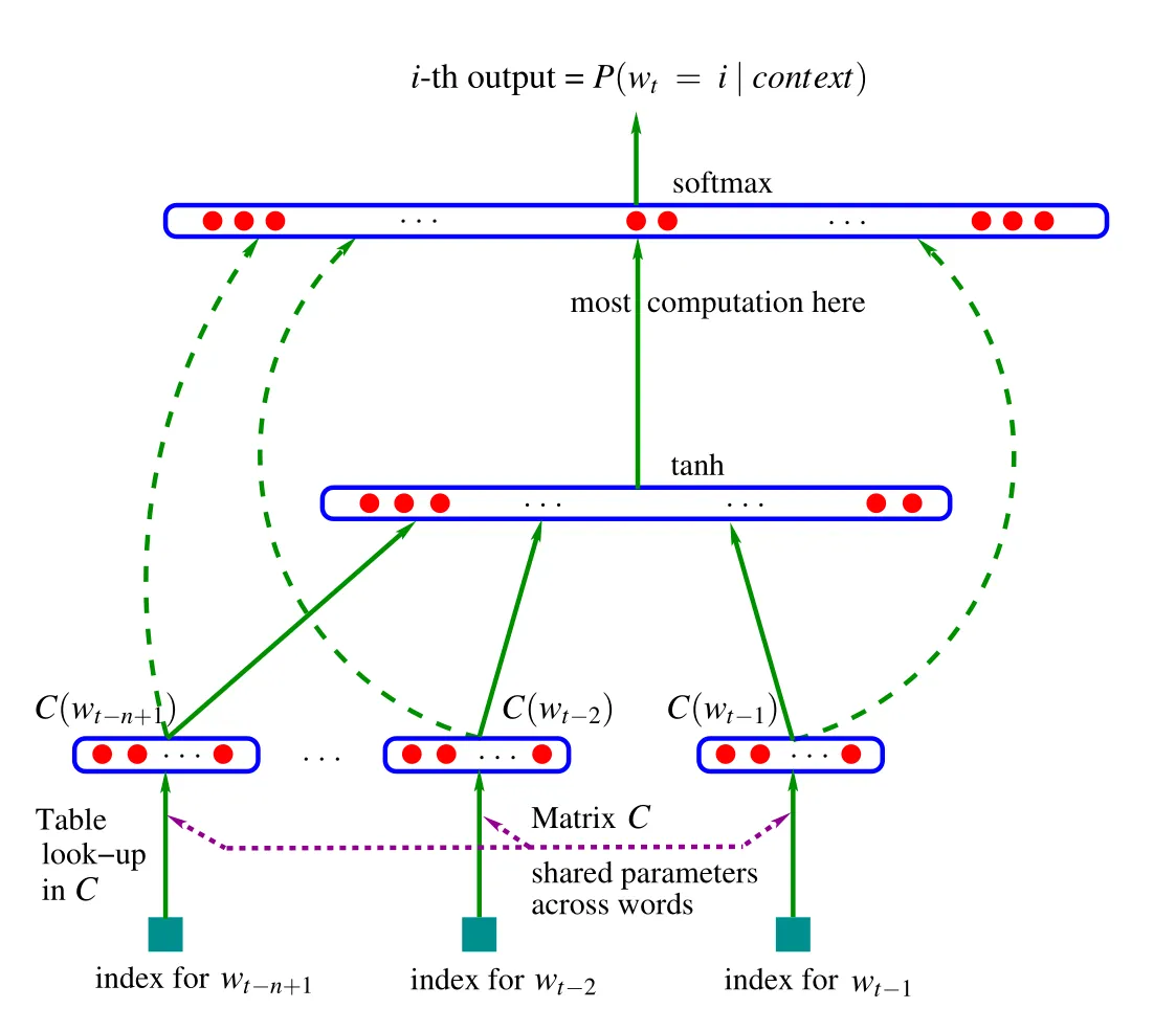
The context for this word-level language model is 3 previous words. Each word is converted to an embedding using the table C. C is an embedding lookup table with dimension (vocab_size, embedding_dim). In the paper, vocab_size is 17,000 and embedding_dim is 30.

The input layer has 30 x 3 = 90 neurons, which is the concatenation of the 3 word embeddings.

The hidden layer has 128 fully-connected neurons with tanh activation.

The output layer is 17,000 fully-connected neurons that output the predicted logits for the next word. This goes through a softmax layer to produce a probability distribution from which the next word is sampled.

The parameters are the weights and biases of the output layer, the hidden layer, and the embedding table C.

Training minimizes the negative log-likelihood of the predicted word w.r.t the model parameters, i.e., maximizing the probability of the true next word.

Intuition: Think of the embedding space as a continuous space where words with similar meanings are close to each other. The model can then learn what words appear in similar contexts, even if they didn’t appear in the training set.

Why mini-batch SGD trains faster

Number of epochs is 1000.

Aspect	Mini-Batch (32)	Full-Batch (200K)
Updates per epoch	1	1
Samples processed	32K	200M
Gradient quality	Noisy estimate	Exact

Key takeaways:

1. More updates, less compute: Each mini-batch update moves params toward the solution. Full-batch needs ~6000× more compute for the same # of updates.

2. Noise is a feature, not a bug: Noisy gradients help escape bad local minima and act as regularization.

3. Diminishing returns — Gradient accuracy scales with , so 6250× more samples only gives ~79× better gradient.

Rule of thumb: Larger batch → need more epochs AND often lower learning rate.

Intuition: It’s much better to take more steps with a noisy gradient than fewer steps with an exact gradient.

Exponential vs linear spacing for learning rate search

Problem: Learning rates span orders of magnitude (0.001 → 1.0)

Range	Linear (1000 pts)	Exponential (1000 pts)
0.001–0.01	~9 points	~333 points
0.01–0.1	~90 points	~333 points
0.1–1.0	~900 points	~333 points

Linear spacing = biased toward large values

• 90% of points land in 0.1–1.0
• Only 1% explore 0.001–0.01

Exponential spacing = uniform across scales

• Equal points per decade: 0.001–0.01, 0.01–0.1, 0.1–1.0

Intuition: Use exponential spacing when searching parameters that vary by orders of magnitude (LR, regularization, etc.)

Learning rate search methods

	Grid search	Dynamic sweep
How	Train N separate models	1 run, increase LR each step
Cost	High	Low
Accuracy	Exact	Approximate
Use	Final tuning	Quick ballpark

Workflow: Dynamic sweep → find range → Grid search within range

OR Dynamic sweep → pick best LR → fine-tune with decay schedule

Dataset splits

Standard practice is to split dataset into 3 parts:

• Training set: used to train the model, do backprop, update weights
• Dev/validation set: used to tune hyperparameters during development (e.g., learning rate, architecture, etc.)
• Test set: used to evaluate final model performance after training is complete

Weight initialization

Intuition: At init, if the predicted logits are all roughly the same, the loss (negative log likelihood) will be small. However, if the logits have extreme values, the loss can be very high and sometimes reach inf. We can avoid this by scaling the weights and biases by a small value.

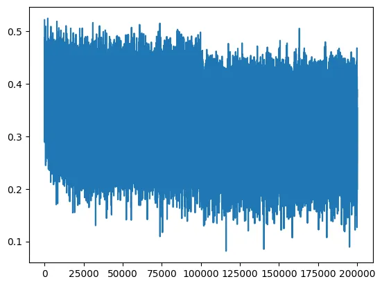
Hockey stick loss plot: it seems like you’re making good gains at the beginning, but that’s just a symptom of bad weights initialization. As the neural network learns the first few steps, it squashes down the weights, exactly what we do above. So these are easy gains and we humans can pre-do it at init.

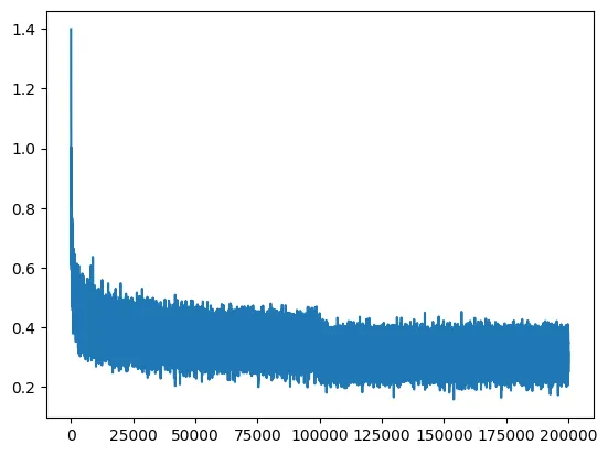
And below is a plot of what happens when we initialize weights correctly and the neural network has to learn the hard gains.

This way, the network spends more cycles optimizing and reducing loss rather than fixing bad initialization.

The flat regions of activation functions

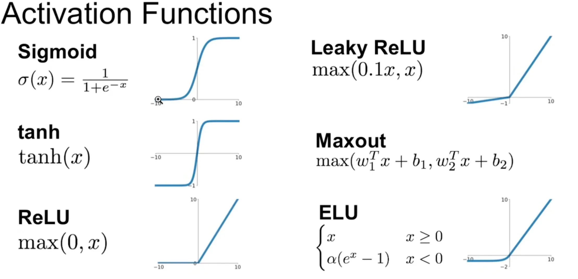
Lots of activation functions have flat regions where the gradient is close to 0. If a neuron’s input falls into this region, the neuron will not learn because gradient descent will not update its weights. If no input examples can activate a neuron and make it learn, it is called a “dead neuron”.

Other times, a too high learning rate might knock a neuron’s input into the flat region, killing it. From that point on, the neuron will never recover because it will not learn on any input -> permanent brain damage to the network.

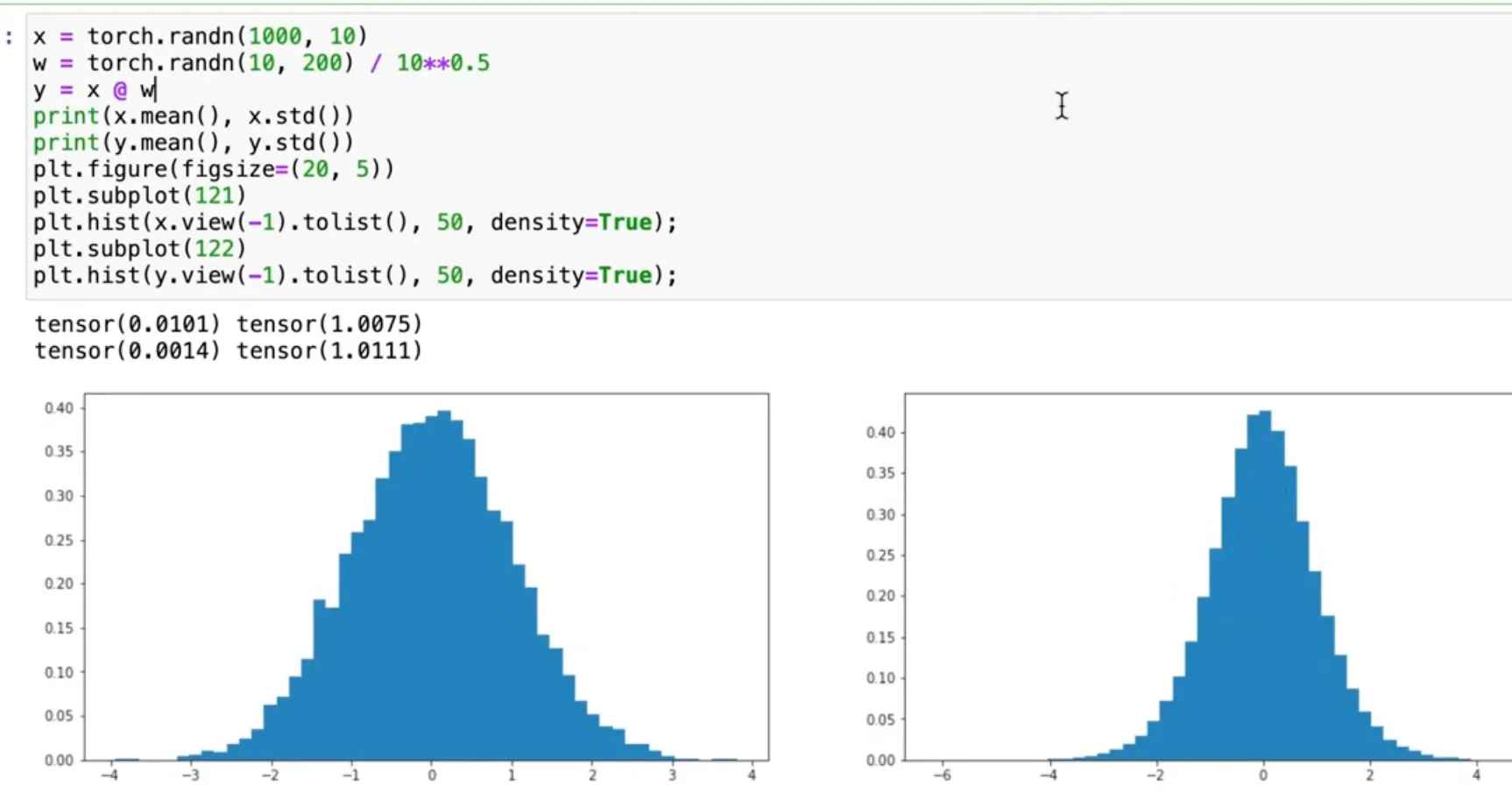
Good weight initialization

Intuition: input set is assumed to have Gaussian distribution with mean 0 and std 1. We want to initialize weights so that each layer’s pre-activation output also have mean 0 and std 1. This prevents activations from falling into flat regions (i.e., “well-behaved”).

One way to do this is to scale weights and biases by a small value at init like so.

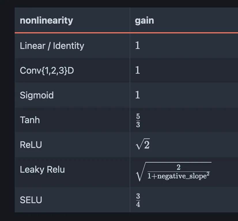
One paper delved deep into this: “Delving Deep into Rectifiers: Surpassing Human-Level Performance on ImageNet Classification” by He et al., 2015.

Key idea is because ReLU zeroes out half the inputs, we need to scale weights by with being the number of input connections to the layer. The gain factor is 2 because half the inputs are zeroed out by ReLU. For tanh, it’s .

Even after the Kaiming paper, weight initialization and nonlinearities chosen and plotting out ranges of activations, etc. Everything is still very fragile for the neural network to train. However some modern innovations for stable training without initialization tricks are:

• Residual connections (ResNets)
• Normalization layers (BatchNorm, LayerNorm, GroupNorm, etc.)
• Much better optimizers (RMSProp, Adam, etc.)

BatchNorm

From “Batch Normalization: Accelerating Deep Network Training by Reducing Internal Covariate Shift” by Ioffe and Szegedy, 2015.

Key idea is instead of fiddling with scaling to wish for a well-behaved preactivation, we can just normalize the pre-activation output of each layer to be Gaussian. Sounds kind of crazy but it works because standardizing the inputs to be Gaussian is a perfectly differentiable operation, so gradients can still flow.

Mechanism: for each batch, compute the mean and std of the pre-activation output, then standardize it. However, we don’t want to always force it to be Gaussian at all times. The neural network should be allowed to learn to shift and scale the normalized output around. To do this, we add 2 learnable parameters per layer, gain and bias, that scale and shift the normalized output.

However, at inference time, we don’t have batches. So the paper suggests keeping a running mean and std to use at inference time.

Weak point: BatchNorm couples the training to the batch size because the mean and std are derived from the batch. Not undesirable though as this is a form of data augmentation as it introduces noise to the activations from other examples in the batch. However, people have tried to decouple it with techniques like GroupNorm, LinearNorm, etc.

Best practice: Append BatchNorm after linear/conv layer and before nonlinearity. Remove bias from linear/conv layer since BatchNorm effectively subtracts from the mean.

Observing training

When training a neural network, it’s important to observe:

1. Forward pass activations for each layer: are they well-behaved (not too large/small, not in flat regions of nonlinearity)?
2. Backward pass gradients for each layer: are they well-behaved (not too large/small)?
3. Parameter activation and gradient statistics: are weights and biases changing too large/small due to learning rate (update:data ratio)?