Autograd

Backpropagation

An algorithm that evaluates gradient of the loss function with respect to the neural network’s weights. Allows you to minimize loss function by iteratively tune the weights, improving accuracy of network.

Originated in 1964, it doesn’t involve neural network, but happens to be useful so people use it for training NNs.

In the context of neural networks, backprop is only meaningful when training using loss (i.e., gradient descent technically). There are many other training methods that don’t rely on loss function, and thus backprop.

How it works

Backprop works in 2 phases:

1. The forward pass: traces the operations performed on the tensors and constructs a computational DAG
2. The backward pass: traverses the DAG from the output node to the input nodes, recursively applying the chain rule to compute gradients.

This information is crucial as it allows us to see how much the inputs are affecting the outputs:

Backprop starts by seeding the output node’s gradient to 1.0, then build out the computation graph in topological order, and then applying the chain rule to compute gradients for each node. The topo sort is important because it ensures that when we compute the gradient for a node, all of its children have already been computed.

The chain rule

Wikipedia

Tensors

Biggy arrays of scalars, packed together for efficiency when training on GPUs. Not useful for demonstrating backprop, so we only support scalars in darggrad.

Neurons

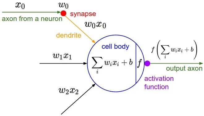
The dot product reveals how much two vectors point in the same direction. If the dot product is zero, the vectors are perpendicular.

Multiple dot products (converting vector x vector to a scalar value) of inputs and weights (synaptic strengths of the input path) go into the weighted sum, offset by a bias (“trigger happiness” of a neuron), and put through an activation function. The activation function is typically a squashing function that limits the output to a certain range, such as between 0 and 1 (sigmoid) or between -1 and 1 (tanh). This helps to introduce non-linearity into the model, allowing it to learn more complex patterns. The loss function measures how far the neuron’s output is from the desired output and is applied to the output during training.

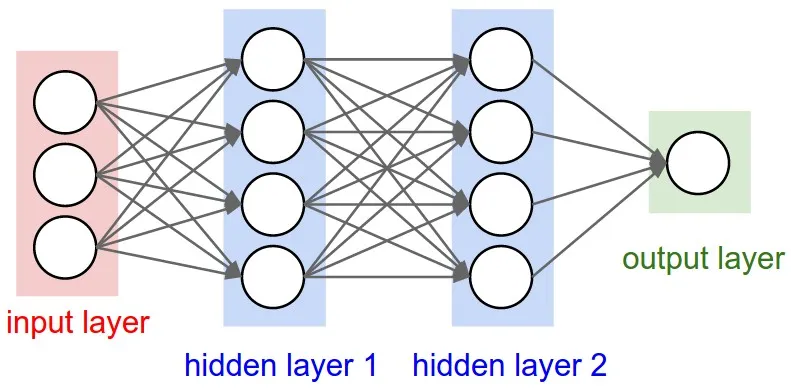
In a neural network, there are many neurons like so organized in layers.

When applied to the context of backprop, we are most interested in how the loss is affected by the neuron’s weights.

Multi-layer perceptron (MLP)

A simple type of neural network where neurons are organized in layers, and each neuron in one layer is connected to every neuron in the next layer.

Basic training loop

1. Have a set of inputs
2. Initialize network weights and biases (parameters)
3. Perform a forward pass to compute the output, and subsequently the loss
4. IMPORTANT: Flush the gradients of all parameters to zero to make sure we don’t accumulate gradients from previous iterations
5. Perform a backward pass to compute gradients of the loss with respect to each parameter
6. Update each parameter value using their gradient and a set learning rate (although a scheduler is often used to adjust the learning rate over time according to the loss trajectory during training)
7. Perform steps 3-5 for many iterations until the loss is minimized

Design decision tidbits

Why wrap Value in shared and mutable smart pointer.

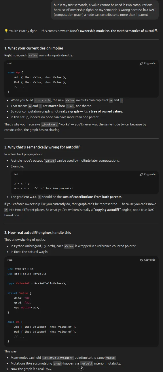
Choosing between Box, Arc, Rc, Cell, RefCell, Mutex.

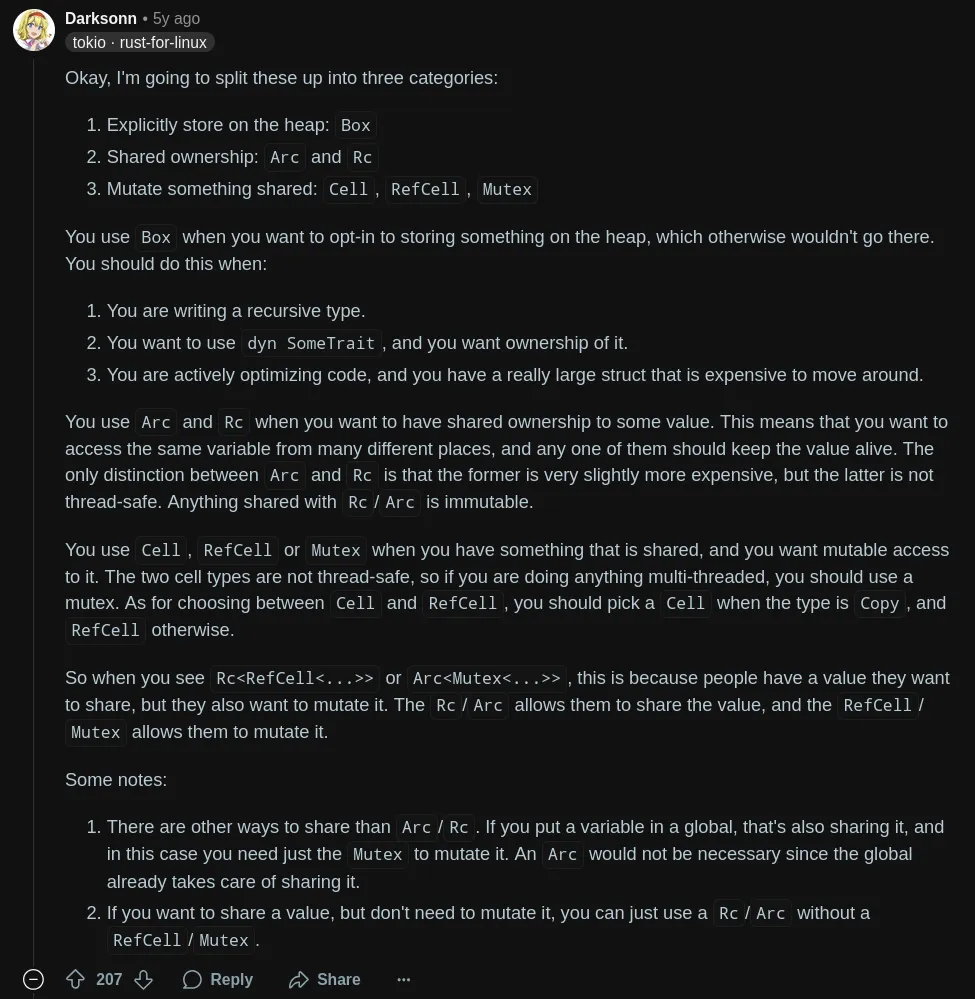
We use Rc<RefCell<Value>> for simplicity (shared, single-threaded, mutable through interior mutability).

In PyTorch, you have to declare that a leaf node requires gradient (.requires_grad = True). PyTorch doesn’t track gradients on leaf nodes for efficiency reasons.